Introduction to Quantum Error Correction

#lecture #quantum-error-correction #stabilizer-codes #fault-tolerance

Introduction

Over the past weeks, we have covered the two ends of the quantum computing stack.
We started with the physical platforms: neutral atoms trapped, trapped ions, superconducting circuits, photons, and quantum dots.
We then moved to quantum algorithms.
We studied Shor's factoring algorithm, we explored Grover's search algorithm and its quadratic speedup through amplitude amplification.
We also confronted the resource estimation reality check: factoring a 2048-bit RSA key requires millions of physical qubits and hours/days of coherent operation, far beyond what any current device can provide.

The gap between the error rates of today's physical qubits and the requirements of fault-tolerant algorithms is the central challenge of the field.
This is not a nice-to-have problem: it is the bottleneck standing between quantum computing theory and reality.

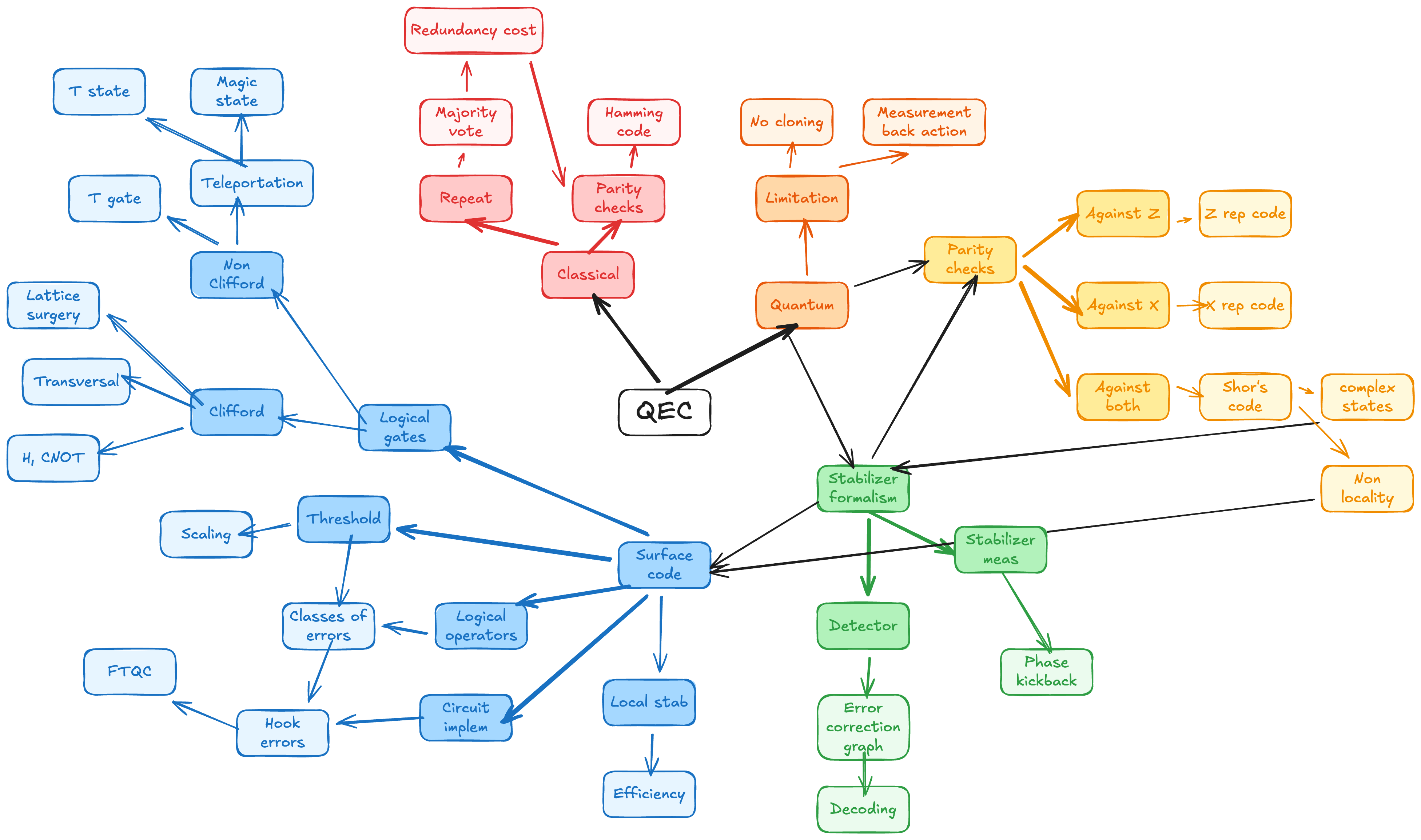
Today's lecture addresses this gap with Quantum Error Correction (QEC).
We will see how to protect fragile quantum information from noise by encoding it redundantly across many physical qubits, creating robust logical qubits.
We begin with classical error correction to build intuition, then confront the unique challenges of the quantum world (eg the No-Cloning Theorem, measurement back-action), and progressively build up from simple repetition codes, the most classical of QEC codes, to the Shor code, the stabilizer formalism, and finally the surface code.
We will also discuss fault-tolerant circuit design, logical gates, and the threshold theorem that guarantees error correction works even with imperfect components.

These notes were written for the Experimental Quantum Computing and Error Correction course of M2 Master QLMN, see the course's website for more information.

For next time 2026-02-18

You are not expected to solve any exercice from today's lecture.
Instead, read Acharya et al, Quantum error correction below the surface code threshold, 2025 (https://www.nature.com/articles/s41586-024-08449-y) 1.
We'll discuss it during next lecture.

Quiz: Exponential Suppression of Errors in QEC

Let's begin by discussing the paper from Google Quantum AI team untitled "Exponential suppression of bit or phase errors with cyclic error correction." Nature 595, 383-387 (2021). DOI: 10.1038/s41586-021-03588-y 2.
Here are 5 questions to check our understanding.

Q1: Code Implementation

Which quantum error correction code structure was primarily implemented to demonstrate the exponential suppression of errors in this experiment?

A. A 2D surface code measuring both $X$ and $Z$ stabilizers simultaneously to correct all errors.

B. A 1D repetition code embedded in a 2D grid, configured separately for either bit-flip or phase-flip protection.

C. A Shor code encoding 1 logical qubit into 9 physical qubits.

D. A bosonic cat code using superconducting cavities.

Answer

Correct Answer: B

The experiment implemented a 1D repetition code embedded in the 2D Sycamore chip grid.
The code was configured separately for bit-flip protection (using $Z_{i} Z_{i + 1}$ stabilizers) or phase-flip protection (using $X_{i} X_{i + 1}$ stabilizers), but not both simultaneously.

Q2: Logical Error Scaling

According to the experimental results, how does the logical error probability per round ( $ϵ_{L}$ ) scale with the code distance $d$ ?

A. Linearly: $ϵ_{L} \propto 1 / d$

B. Quadratically: $ϵ_{L} \propto 1 / d^{2}$

C. Exponentially: $ϵ_{L} \propto Λ^{- d / 2}$ where $Λ$ is the error suppression factor.

D. The logical error rate remained constant as $d$ increased due to correlated noise.

Answer

Correct Answer: C

The main result of the paper is the exponential suppression of logical errors with code distance.
$Λ > 1$ means each additional pair of qubits suppresses the error by a constant factor, demonstrating below-threshold operation.

Q3: Experimental Parameters

Which of the following correctly describe the scale of the repetition code experiments performed? (Select all that apply)

A. The code distances ranged from $d = 3$ to $d = 11$ .

B. The largest code used 21 superconducting qubits (11 data qubits, 10 measure qubits).

C. The experiment was limited to $d = 3$ due to chip size constraints.

D. The logical error suppression was shown to be stable over 50 rounds of error correction.

Answer

Correct Answers: A, B, D

The experiment demonstrated codes from $d = 3$ to $d = 11$ using up to 21 qubits, and showed stable suppression over 50 rounds.
The Sycamore chip had sufficient qubits to go well beyond $d = 3$ .

Q4: Error Handling Configuration

How did the experiment address the distinction between bit-flip and phase-flip errors? (Select all that apply)

A. A single surface code patch corrected both error types concurrently.

B. The "Phase-Flip Code" used $X_{i} X_{i + 1}$ stabilizers to detect $Z$ errors.

C. The "Bit-Flip Code" used $Z_{i} Z_{i + 1}$ stabilizers to detect $X$ errors.

D. Phase-flip errors were found to be negligible compared to bit-flip errors.

Answer

Correct Answers: B, C

The experiment ran two separate configurations.
The bit-flip code measured $Z_{i} Z_{i + 1}$ parity to catch $X$ errors, while the phase-flip code measured $X_{i} X_{i + 1}$ parity to catch $Z$ errors.
Each configuration protects against only one error type at a time.

Q5: Physical Error Model

What conclusion did the authors reach regarding the physical error mechanisms in the device?

A. The errors were dominated by non-local cosmic ray events that destroyed the code immediately.

B. The device performance was well-described by a simple uncorrelated depolarizing error model.

C. $T_{1}$ relaxation was the sole limiting factor for both bit and phase codes.

D. Correlated errors were significant enough to prevent any error suppression as distance increased.

Answer

Correct Answer: B

The paper found that the device noise was well-modeled by simple uncorrelated Pauli errors, which is why the exponential suppression with distance was observed.
Correlated errors were present but subdominant.

Classical Error Correction

Before diving into the quantum realm, let's build intuition from the classical world.
To understand why we need quantum codes, we first need to appreciate how we protect classical information from noise.
This section draws inspiration from the foundational concepts of information theory ?.

The Noisy Channel

Imagine we want to send a single bit of information, either a $0$ or a $1$ , through a communication line.
In a perfect world, what you send is what you get.
But physical systems are rarely perfect.
We face two primary challenges:

Transmission Noise: Sending a bit via a noisy line where there is a non-zero probability that the bit flips during transit.
Storage Decay: Storing a bit in memory where, over time, thermal fluctuations or cosmic rays might cause the bit to flip with a probability $p$ .

The question is: How can we increase the chance of successful transmission or storage despite this inherent noise?

Redundancy and the Majority Vote

The most intuitive solution is redundancy.
If a single bit is fragile, why not use many?
This is the core idea behind the Classical Repetition Code.
Instead of storing a single bit, we store multiple copies of that same bit and periodically perform a "sanity check" using a Majority Vote algorithm.

The Idealized Assumption

For this introductory derivation, we assume that the process of "reading" the bits to take a majority vote is itself perfect and instantaneous.
We are only concerned with the errors occurring in the bits themselves during the "waiting" or "traveling" periods.

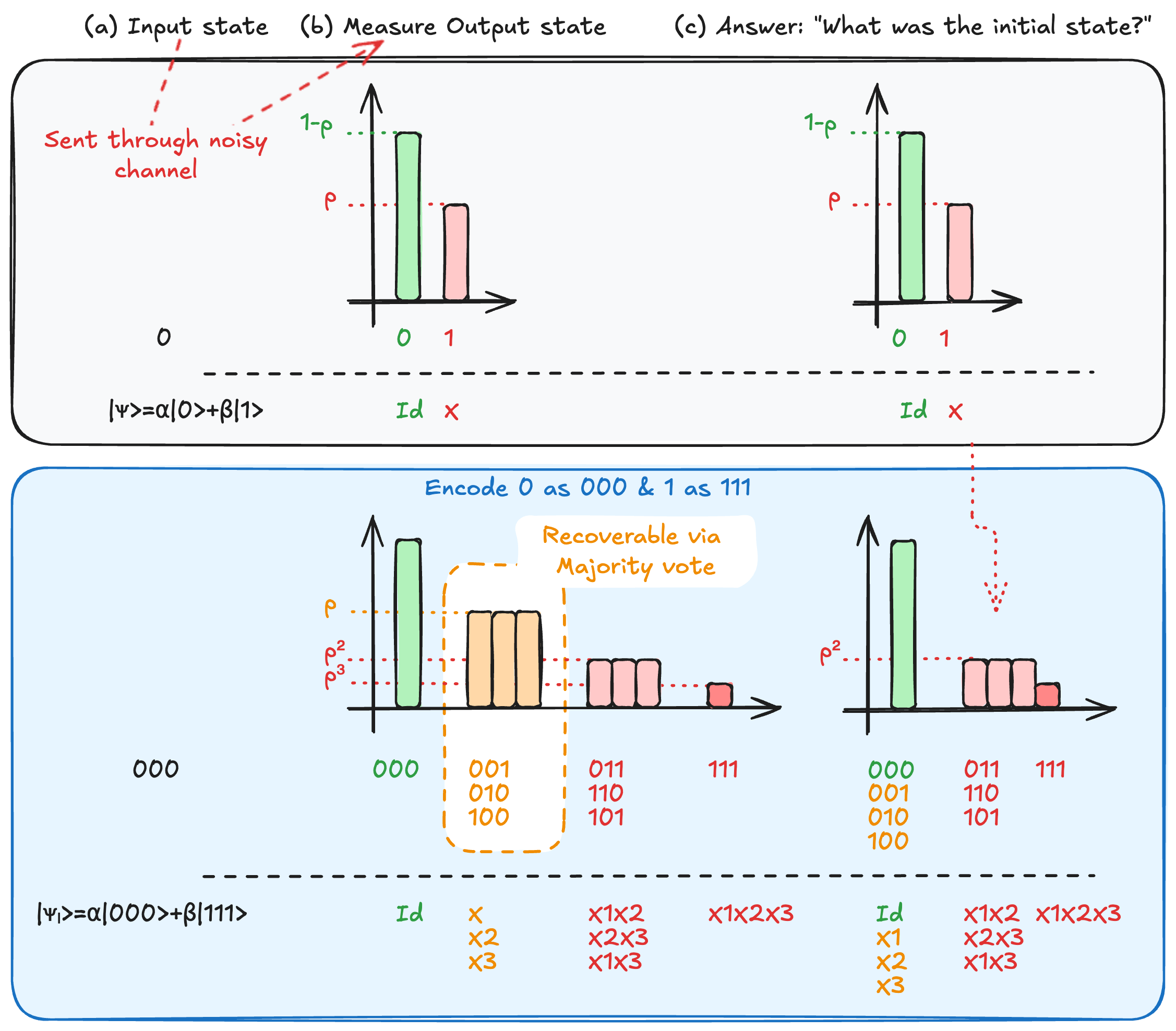
If we use 3 bits to represent a single logical $0$ (encoded as $000$ ), we can tolerate one error.
If a single bit flips to $1$ (e.g., $010$ ), the majority is still $0$ , and we can "correct" the state back to $000$ .
However, if two bits flip, the majority vote fails, and we incorrectly conclude the logical bit was a $1$ .
This error suppression mechanism is illustrated in Fig..

Error suppression in the 3-qubit repetition code: comparison of error probabilities between an unencoded single qubit (top) and a logical qubit encoded as (bottom). The repetition code allows recovery from all single-bit errors via majority vote decoding, suppressing the logical error rate to .|600 — Error suppression in the 3-qubit repetition code: comparison of error probabilities between an unencoded single qubit (top) and a logical qubit encoded as ${| 0 ⟩}_{L} = | 000 ⟩$ (bottom). The repetition code allows recovery from all single-bit errors via majority vote decoding, suppressing the logical error rate to $O (p^{2})$ .

Lexicon and Definitions

To speak the language of error correction, we must define two critical terms:

Logical States: These are the "effective" qubit states we care about. Remember that for a physical qubit also, we emphasised that qubit states do not exist, they are encoded in physical Hilbert space. For a repetition code, we thus define:
- $0_{L} = 000 \dots 0$
- $1_{L} = 111 \dots 1$
Code Distance ( $d$ ): This is the minimal number of physical bit flips required to transform a valid $0_{L}$ into a valid $1_{L}$ .
- For a 3-bit code ( $d = 3$ ), you need 3 flips to go from $000$ to $111$ .
- For a 5-bit code ( $d = 5$ ), you need 5 flips.

Intuition: Code Distance and Correction Power

A code with distance $d$ can correct any $t$ errors as long as those errors do not flip the majority.
Mathematically, the code fails only if at least $\frac{d + 1}{2}$ errors occur.
So a distance- $d$ code corrects up to $t = ⌊ \frac{d - 1}{2} ⌋$ errors.
Furthermore, there is a distinction between detecting and correcting errors.
A code can detect up to $d - 1$ errors (since the state is no longer a valid codeword), but it can only safely correct up to $⌊ \frac{d - 1}{2} ⌋$ .

Error Suppression Scaling

If the probability of a single bit flipping is $p$ , then for a $d = 3$ code, the failure probability scales as $O (p^{2})$ .
For a $d = 5$ code, it scales as $O (p^{3})$ .
As long as $p < 0.5$ , increasing the redundancy significantly suppresses the logical error rate.
This exponential suppression with distance is the whole point of error correction.

Exercise 1: Repetition Code Failure Probability

Consider a classical $d = 5$ repetition code with single-bit error probability $p = 0.01$ .

Calculate the probability that the majority vote fails (i.e., 3 or more out of 5 bits flip).
Compare this to the uncoded error probability $p = 0.01$ .
What is the ratio of encoded to unencoded error probability? What does this tell you about the value of redundancy?

Answer

The majority vote fails when 3, 4, or 5 bits flip.
Using the binomial distribution:

P_{fail} = (\binom{5}{3}) p^{3} (1 - p)^{2} + (\binom{5}{4}) p^{4} (1 - p) + (\binom{5}{5}) p^{5}

= 10 \times (0.01)^{3} \times (0.99)^{2} + 5 \times (0.01)^{4} \times 0.99 + (0.01)^{5}

\approx 10 \times 10^{- 6} \times 0.98 + 5 \times 10^{- 8} \times 0.99 + 10^{- 10}

\approx 9.8 \times 10^{- 6}

The unencoded error probability is $p = 0.01 = 10^{- 2}$ .
The ratio is approximately $10^{- 6} / 10^{- 2} = 10^{- 4}$ .
The 5-bit code suppresses the error rate by four orders of magnitude.
Redundancy pays off when $p$ is small.

The Cost of Redundancy

While redundancy grants us protection, it is not free.
We must consider the resource overhead.
If we want to encode $k$ logical bits into $n$ physical bits, we define the Code Rate as $R = k / n$ .

Metric	Calculation	Value
Data ( $k$ )	The original information	4 bits
Encoded ( $n$ )	Total physical bits ( $4 \times 3$ )	12 bits
Redundancy	$n - k$	8 bits
Rate ( $R$ )	$k / n$	$1 / 3$

The physical scaling is linear: if you have $1$ Terabyte of data to protect, you would need $3$ Terabytes of storage.
The efficiency of the encoding becomes a challenge.
We have seen that we can achieve high protection by increasing $d$ , but this usually forces the Rate $k / n$ to plummet.
The question becomes how can we increase the Rate ( $R$ ) or decrease the redundancy required while maintaining the same level of protection?
This question leads us directly into the world of Linear Codes and, eventually, Quantum Error Correcting Codes.

Hamming Code: Parity and the Price of Information

In the 1940s at Bell Labs, Richard Hamming was frustrated by the fragility of electromechanical computers, which frequently crashed due to bit flips.
Here is an excerpt of the Hamming code Wikipédia page:

Hamming worked on weekends, and grew increasingly frustrated with having to restart his programs from scratch due to detected errors.
In a taped interview, Hamming said, "And so I said, 'Damn it, if the machine can detect an error, why can't it locate the position of the error and correct it?'".

This led to the development of the Hamming Code, a method of checking the parity of data bits to increase the reliability (the rate) of information transfer.
The idea behind Hamming codes is to add a specific number of redundant bits, which we often call ancilla bits (specifically in the context of our QEC circuits).
These ancilla bits allow us to detect that an error has occurred and uniquely identify where (on which data qubit) it happened.

Geometric Intuition: The Hamming(7,4) Code

Consider $k = 4$ data bits, labeled $d_{1}, d_{2}, d_{3}, d_{4}$ .
To protect these, we add three parity bits: $p_{1}, p_{2}, p_{3}$ .
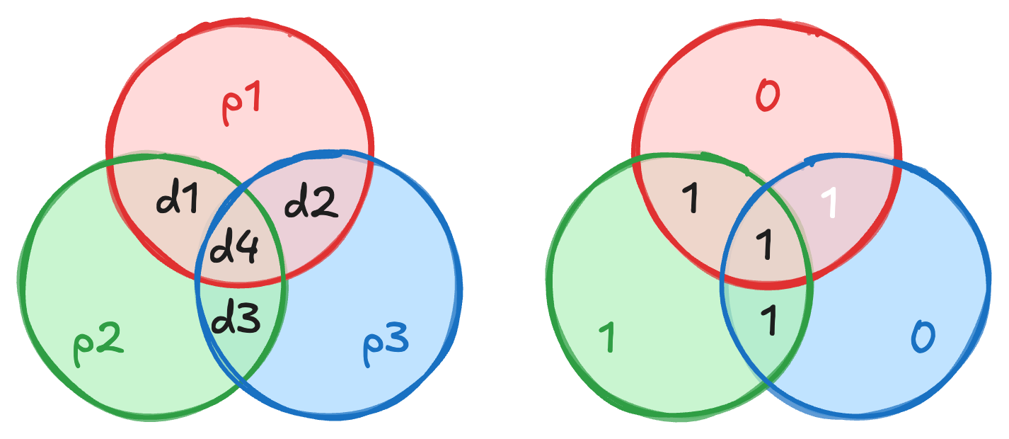
A good way to visualize this is through a Venn diagram where the four data bits sit in the intersections of three overlapping circles, see Fig..
Each parity bit is responsible for maintaining an even parity within its respective circle:

$p_{1}$ is the parity of $d_{1}, d_{2},$ and $d_{4}$ .
$p_{2}$ is the parity of $d_{1}, d_{3},$ and $d_{4}$ .
$p_{3}$ is the parity of $d_{2}, d_{3},$ and $d_{4}$ .

Venn diagram representation of the Hamming(7,4) code. Data bits sit at the intersections of three circles, with parity bits controlling each circle. When data has an error on , parity checks and fail while remains correct, uniquely identifying .|500 — Venn diagram representation of the Hamming(7,4) code. Data bits sit at the intersections of three circles, with parity bits controlling each circle. When data $1011$ has an error on $d_{2}$ , parity checks $p_{1}$ and $p_{3}$ fail while $p_{2}$ remains correct, uniquely identifying $d_{2}$ .

We can also represent this relationship using a parity-check matrix where each row shows which data bit is involved in a given parity bit:

Parity	$d_{1}$	$d_{2}$	$d_{3}$	$d_{4}$
$p_{1}$	x	x		x
$p_{2}$	x		x	x
$p_{3}$		x	x	x

Parity Logic

Mathematically, we define the parity such that the sum (modulo 2) of the bits in a circle is zero.
For example, $p_{1} \oplus d_{1} \oplus d_{2} \oplus d_{4} = 0$ .

Error Identification and the Syndrome

What makes this data+parity bits system work is univocal identification.
If any given data bit flips, it will change the parity of the specific circles it belongs to such that by reading the set of parity violations, also called the syndrome, we obtain an "error location address" that tells us where the error occurred.

Suppose our data is $1011$ and an error occurs on $d_{2}$ .
We would observe that the new values of the parity checks associated with $p_{1}$ and $p_{3}$ fail (they were initially 0, but should be 1 after the error), while $p_{2}$ remains correct.
Looking at our map, $d_{2}$ is the only bit shared exclusively by $p_{1}$ and $p_{3}$ , pointing us directly to the source of the error.
From a linear algebra perspective, this is handled by the Code Generator Matrix.

Looking back at our redundancy table, while a simple repetition code (1 data bit with 2 "copy" ancilla bits) provides high redundancy but low efficiency, the Hamming(7,4) code strikes a balance.
With $n = 7$ total bits and $k = 4$ data bits, we have a rate of $R = 4 / 7 \approx 0.57$ almost two as big as the previous encoding rate.
This scaling is efficient: the redundancy grows only as $\log k$ (compared to linear).

Exercise 2: Hamming Code Syndrome Calculation

Consider a Hamming(7,4) code with data bits $d_{1} d_{2} d_{3} d_{4} = 1101$ and parity bits computed as described above.

Compute the three parity bits $p_{1}, p_{2}, p_{3}$ .
Suppose $d_{3}$ is flipped. What syndrome do you observe (which parity checks fail)?
Verify that the syndrome uniquely identifies $d_{3}$ as the corrupted bit.

Answer

With $d_{1} = 1, d_{2} = 1, d_{3} = 0, d_{4} = 1$ :
- $p_{1} = d_{1} \oplus d_{2} \oplus d_{4} = 1 \oplus 1 \oplus 1 = 1$
- $p_{2} = d_{1} \oplus d_{3} \oplus d_{4} = 1 \oplus 0 \oplus 1 = 0$
- $p_{3} = d_{2} \oplus d_{3} \oplus d_{4} = 1 \oplus 0 \oplus 1 = 0$
If $d_{3}$ flips ( $0 \to 1$ ), recompute parities:
- $p_{1}$ : $d_{1} \oplus d_{2} \oplus d_{4} = 1 \oplus 1 \oplus 1 = 1$ (unchanged, $p_{1}$ passes)
- $p_{2}$ : $d_{1} \oplus d_{3}^{'} \oplus d_{4} = 1 \oplus 1 \oplus 1 = 1 \neq 0$ ( $p_{2}$ fails)
- $p_{3}$ : $d_{2} \oplus d_{3}^{'} \oplus d_{4} = 1 \oplus 1 \oplus 1 = 1 \neq 0$ ( $p_{3}$ fails)
- Syndrome: $p_{1}$ OK, $p_{2}$ FAIL, $p_{3}$ FAIL.
Looking at the parity-check matrix, $d_{3}$ participates in $p_{2}$ and $p_{3}$ but not $p_{1}$ . This matches the observed syndrome, uniquely identifying $d_{3}$ .

From Classical to Quantum: The Measurement Back-Action

As we move from the classical regime to the quantum one, the motivation for encoding via parity bits changes fundamentally.
In the classical world, adding parity encoding ancilla bits is an efficiency-driven choice: we do it to avoid the cost of re-calculating or re-storing data.

In the quantum world, however, encoding data parity in parity storing ancilla qubits becomes a physical necessity.
This is due to two things: the No-cloning theorem that says that we cannot simply clone aka copy quantum states (said in another way, there is no unitary operation $U$ such that $U | ψ ⟩ | 0 ⟩ = | ψ ⟩ | ψ ⟩$ for all $| ψ ⟩$ ) and the "measurement Back action" problem.
This last one implies that if we were to measure our data qubits encoding an arbitrary quantum state directly to check for errors, we would collapse their superposition, destroying the very quantum information we are trying to protect.
Instead, we must map the parity information onto ancilla qubits and measure only those, allowing us to extract the syndrome without "touching" the data itself.
This insight is at the heart of the stabilizers, as established in the foundational work of 3 and that we will discuss after looking at simpler examples first.

Exercise 3: Code Rate Comparison

Compare the code rate $R = k / n$ for the following classical codes:

A 3-bit repetition code encoding 1 logical bit.
A Hamming(7,4) code encoding 4 logical bits.
A Hamming(15,11) code encoding 11 logical bits.
What general trend do you observe? Why is this relevant for quantum codes?

Answer

$R = 1 / 3 \approx 0.33$
$R = 4 / 7 \approx 0.57$
$R = 11 / 15 \approx 0.73$
The rate increases as we encode more data bits with the Hamming family.
The number of parity bits grows as $\log_{2} (n + 1)$ , so the overhead becomes a smaller fraction.
For quantum codes, this trade-off is even more critical because each physical qubit is expensive (in terms of hardware and control), making high-rate codes desirable.

Exercise 4: No-Cloning Theorem

Assume a unitary $U$ exists such that $U | 0 ⟩ | 0 ⟩ = | 0 ⟩ | 0 ⟩$ and $U | 1 ⟩ | 0 ⟩ = | 1 ⟩ | 1 ⟩$ .
Apply $U$ to the state $| + ⟩ | 0 ⟩ = \frac{1}{\sqrt{2}} (| 0 ⟩ + | 1 ⟩) | 0 ⟩$ and show that the result is not $| + ⟩ | + ⟩$ .

Answer

By linearity of $U$ :

U | + ⟩ | 0 ⟩ = \frac{1}{\sqrt{2}} (U | 0 ⟩ | 0 ⟩ + U | 1 ⟩ | 0 ⟩) = \frac{1}{\sqrt{2}} (| 00 ⟩ + | 11 ⟩)

This is a Bell state (maximally entangled), not the product state $| + ⟩ | + ⟩ = \frac{1}{2} (| 00 ⟩ + | 01 ⟩ + | 10 ⟩ + | 11 ⟩)$ .

A machine that correctly copies $| 0 ⟩$ and $| 1 ⟩$ cannot correctly copy $| + ⟩$ .
No single unitary can clone all states, so a universal quantum cloning machine is impossible.
This is why quantum error correction must use entanglement rather than copying.

Quantum Repetition Code

To bypass the measurement problem, we use a Repetition Code that follows the key concepts of the classical one but tailored for quantum states.
While this code only protects against one type of error at a time, specifically bit-flips ( $X$ errors) or phase-flips ( $Z$ errors), it introduces the concept of Quantum Parity Measurements.

Instead of checking the value of qubit 1 and then qubit 2, we ask a relational question, just like in Hamming codes: "Are these two qubits the same or different?"
This question has a binary answer: $0$ for same like in $| 00 ⟩$ and $| 11 ⟩$ , $1$ for different, as in $| 01 ⟩$ and $| 10 ⟩$ .
This tells us if an error occurred without revealing whether the qubits are in state $| 0 ⟩$ or $| 1 ⟩$ .
Said in another way, if we consider a general 2-qubit state:

| ψ ⟩ = α | 00 ⟩ + β | 01 ⟩ + γ | 10 ⟩ + δ | 11 ⟩

Measuring the qubits $Z_{1}$ and $Z_{2}$ individually, we would gain too much information.
For instance, if we found $Z_{1} = + 1$ and $Z_{2} = - 1$ , the state would collapse specifically to $| 01 ⟩$ .

The 3-Qubit Bit-Flip Code

To build our intuition, let's look at the simplest possible instance: protecting against a single bit-flip error ( $X$ gate).
Again, we borrow the classical idea of redundancy but adapt it to the quantum regime.
We define our logical basis states by the mapping:

\begin{aligned} {| 0 ⟩}_{L} & = | 000 ⟩ \\ {| 1 ⟩}_{L} & = | 111 ⟩ \end{aligned}

An arbitrary physical state $| ψ ⟩ = α | 0 ⟩ + β | 1 ⟩$ is now a logical state ${| ψ ⟩}_{L} = α | 000 ⟩ + β | 111 ⟩$ spread across three physical qubits.
If a bit flip occurs on the first qubit, the state becomes $α | 100 ⟩ + β | 011 ⟩$ .
Our parity measurements would reveal that the first and second qubits are different, but the second and third are the same.
Just like in the classical setting, this "syndrome" tells us exactly which qubit flipped, allowing us to apply a corrective $X$ gate.
In the following, we will see what we mean by parity measurements in this context and how to implement it in practice.
Before that we quickly mention how to switch from $X$ to $Z$ protection.

Exercise 5: Bit-Flip Code Stabilizer Action

Consider the logical state ${| ψ ⟩}_{L} = α | 000 ⟩ + β | 111 ⟩$ .

Verify that $Z_{1} Z_{2} {| ψ ⟩}_{L} = + 1 {| ψ ⟩}_{L}$ (i.e., this state is in the $+ 1$ eigenspace of $Z_{1} Z_{2}$ ).
An $X$ error occurs on qubit 2.
Compute $Z_{1} Z_{2} (X_{2} {| ψ ⟩}_{L})$ and $Z_{2} Z_{3} (X_{2} {| ψ ⟩}_{L})$ .
What is the syndrome? How do you correct the error?

Answer

$Z_{1} Z_{2} | 000 ⟩ = (+ 1) (+ 1) | 000 ⟩ = | 000 ⟩$ and $Z_{1} Z_{2} | 111 ⟩ = (- 1) (- 1) | 111 ⟩ = | 111 ⟩$ . Therefore $Z_{1} Z_{2} {| ψ ⟩}_{L} = α | 000 ⟩ + β | 111 ⟩ = + 1 {| ψ ⟩}_{L}$ .
$X_{2} {| ψ ⟩}_{L} = α | 010 ⟩ + β | 101 ⟩$ .
- $Z_{1} Z_{2} (α | 010 ⟩ + β | 101 ⟩) = α (+ 1) (- 1) | 010 ⟩ + β (- 1) (+ 1) | 101 ⟩ = - (α | 010 ⟩ + β | 101 ⟩)$
  So $Z_{1} Z_{2}$ gives eigenvalue $- 1$ .
- $Z_{2} Z_{3} (α | 010 ⟩ + β | 101 ⟩) = α (- 1) (+ 1) | 010 ⟩ + β (+ 1) (- 1) | 101 ⟩ = - (α | 010 ⟩ + β | 101 ⟩)$ . So $Z_{2} Z_{3}$ gives eigenvalue $- 1$ .
Syndrome: $(- 1, - 1)$ .
From the syndrome table, this uniquely identifies an error on qubit 2.
We apply $X_{2}$ to correct.

The Phase-Flip Code

With quantum mechanics comes a new type of error: the phase-flip ( $Z$ gate), where $Z | 1 ⟩ = - | 1 ⟩$ , on the equator of the Bloch sphere.
If we apply the same bit-flip code, it fails completely because a $Z$ error on any qubit results in a logical phase-flip ${| ψ ⟩}_{L} = α | 000 ⟩ - β | 111 ⟩$ , which our $Z Z$ parity checks cannot detect.

To solve this, we rotate our basis.
By working in the dual basis ${| + ⟩, | - ⟩}$ (accessible via Hadamard gate), a phase-flip in the computational basis acts as a bit-flip in the $X$ -basis:

\begin{aligned} {| + ⟩}_{L} & = | + + + ⟩ \\ {| - ⟩}_{L} & = | - - - ⟩ \end{aligned}

By measuring the stabilizers $X_{1} X_{2}$ and $X_{2} X_{3}$ , we can detect and correct a single $Z$ error just as we did for $X$ errors in the previous example.
This symmetry between $X$ and $Z$ errors is discussed in 4.

Intuition: The

X

Z

Duality

$Z$ errors in the computational basis look exactly like $X$ errors in the Hadamard basis.
The Hadamard gate $H$ interchanges the two: $H Z H = X$ and $H X H = Z$ .
If you can correct bit-flips, you can correct phase-flips simply by rotating your perspective by 90 degrees on the Bloch sphere.

Exercise 6: Phase-Flip Code

Show that a single $Z_{1}$ error on the state ${| ψ ⟩}_{L} = α | + + + ⟩ + β | - - - ⟩$ is undetectable by the $Z_{1} Z_{2}$ stabilizer.
Show that the same $Z_{1}$ error is detected by the $X_{1} X_{2}$ stabilizer.
Hint: Use the fact that $Z | + ⟩ = | - ⟩$ and $Z | - ⟩ = | + ⟩$ .

Answer

$Z_{1} | + + + ⟩ = | - + + ⟩$ and $Z_{1} | - - - ⟩ = | + - - ⟩$ .
The corrupted state is $α | - + + ⟩ + β | + - - ⟩$ .
In the computational basis, $| + ⟩ = \frac{1}{\sqrt{2}} (| 0 ⟩ + | 1 ⟩)$ and $| - ⟩ = \frac{1}{\sqrt{2}} (| 0 ⟩ - | 1 ⟩)$ .
Computing $Z_{1} Z_{2}$ on this state: both $| - + + ⟩$ and $| + - - ⟩$ are superpositions of computational basis states where qubits 1 and 2 can be anything.
The $Z_{1} Z_{2}$ check measures computational-basis parity, which does not correlate with phase information.
Formally, $[Z_{1} Z_{2}, Z_{1}] = 0$ , so $Z_{1}$ commutes with $Z_{1} Z_{2}$ and cannot be detected.
$X_{1} X_{2} | + + + ⟩ = | + + + ⟩$ (eigenvalue $+ 1$ ).
$X_{1} X_{2} | - + + ⟩ = | - + + ⟩ \cdot (- 1) (+ 1) = - | - + + ⟩$
So $X_{1} X_{2} (Z_{1} | + + + ⟩) = X_{1} X_{2} | - + + ⟩ = (- 1) (+ 1) | - + + ⟩ = - | - + + ⟩$ .
The eigenvalue flipped to $- 1$ , detecting the error.
This works because ${X_{1} X_{2}, Z_{1}} = 0$ (they anti-commute).

Exercise 7: Joint vs. Individual Measurement

Consider the state $| ψ ⟩ = \frac{1}{\sqrt{2}} (| 00 ⟩ + | 11 ⟩)$ (a Bell state).

What happens if you measure $Z_{1}$ individually? What is the post-measurement state for each outcome?
What happens if you measure $Z_{1} Z_{2}$ jointly? What is the post-measurement state?

Answer

Measuring $Z_{1}$ :
- Outcome $+ 1$ (prob. 1/2): state collapses to $| 00 ⟩$ .
- Outcome $- 1$ (prob. 1/2): state collapses to $| 11 ⟩$ .
  In both cases, the superposition is destroyed.
Measuring $Z_{1} Z_{2}$ :
- $Z_{1} Z_{2} | 00 ⟩ = (+ 1) (+ 1) | 00 ⟩ = + | 00 ⟩$
- $Z_{1} Z_{2} | 11 ⟩ = (- 1) (- 1) | 11 ⟩ = + | 11 ⟩$
  Both terms have eigenvalue $+ 1$ , so the measurement returns $+ 1$ with certainty.
  The post-measurement state is still $\frac{1}{\sqrt{2}} (| 00 ⟩ + | 11 ⟩)$ , completely unchanged.

Repetition Code Circuit Implementation

One Parity Measurement

How do we actually measure the parity $Z_{1} Z_{2}$ in practice?
We want to check the joint parity of the $0 / 1$ values on the $Z$ -axis.
Mathematically, this corresponds to the eigenvalue of the joint operator $Z_{1} \otimes Z_{2}$ .
To implement parity measurement, we introduce an ancilla qubit initialized in $| 0 ⟩$ .
By applying CNOT gates controlled by $d_{1}$ and $d_{2}$ onto this ancilla, we map the parity $Z_{1} Z_{2}$ onto the ancilla's state.
If the data qubits are in the same state (both 0 or both 1), the ancilla remains $| 0 ⟩$ .
If they differ, the ancilla flips to $| 1 ⟩$ .
This allows us to "monitor" the state without learning the specific values of $α$ and $β$ .
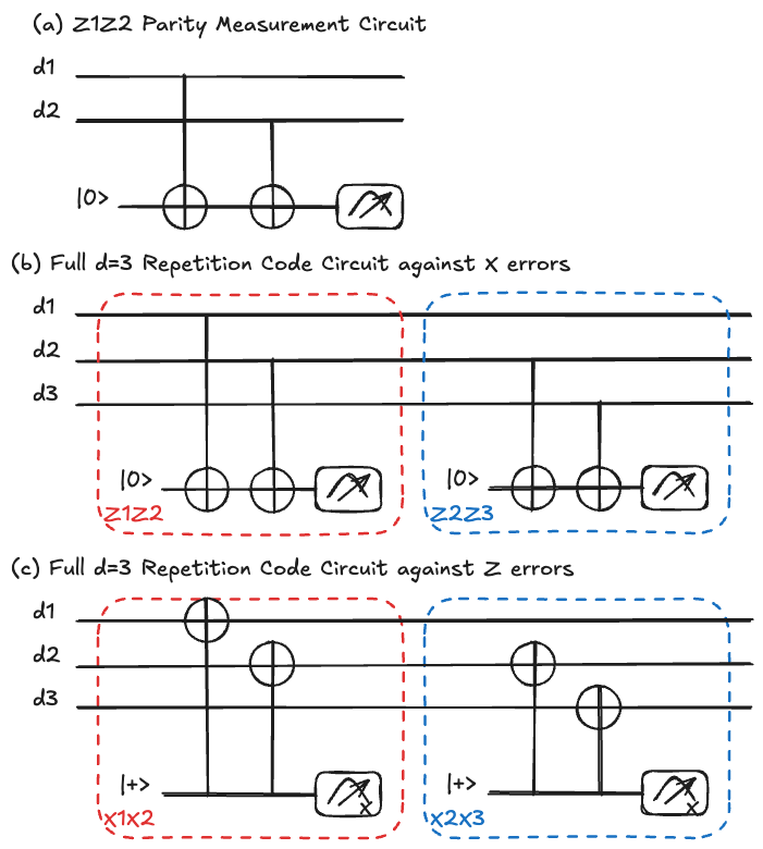
The corresponding circuit is shown in Fig..

a Circuit for a single parity measurement: two CNOT gates controlled by data qubits target a single ancilla, which is then measured. b Full syndrome extraction circuit for the 3-qubit bit-flip code with two ancilla qubits measuring and . c Full syndrome extraction circuit for the 3-qubit phase-flip code with two ancilla qubits measuring and .|600 — a Circuit for a single parity measurement: two CNOT gates controlled by data qubits target a single ancilla, which is then measured. b Full syndrome extraction circuit for the 3-qubit bit-flip code with two ancilla qubits measuring $Z_{1} Z_{2}$ and $Z_{2} Z_{3}$ . c Full syndrome extraction circuit for the 3-qubit phase-flip code with two ancilla qubits measuring $X_{1} X_{2}$ and $X_{2} X_{3}$ .

Exercise 8: Parity Measurement Circuit

Consider the state $| ψ ⟩ = α | 00 ⟩ + β | 11 ⟩$ on data qubits, and an ancilla initialized to $| 0 ⟩$ .

Write the full 3-qubit state before any gates: $| ψ ⟩ {| 0 ⟩}_{a}$ .
Apply CNOT $_{1 \to a}$ (qubit 1 controls, ancilla is target). Write the resulting state.
Apply CNOT $_{2 \to a}$ . Write the resulting state.
What does measuring the ancilla tell you? Does it reveal $α$ or $β$ ?

Answer

$(α | 00 ⟩ + β | 11 ⟩) | 0 ⟩ = α | 000 ⟩ + β | 110 ⟩$
CNOT $_{1 \to a}$ : qubit 1 controls the ancilla flip.
$α | 000 ⟩ + β | 111 ⟩$
(The first $| 0 ⟩$ doesn't flip the ancilla; the first $| 1 ⟩$ in $| 110 ⟩$ flips $| 0 ⟩ \to | 1 ⟩$ .)
CNOT $_{2 \to a}$ : qubit 2 controls the ancilla flip.
$α | 000 ⟩ + β | 110 ⟩$
(In $| 111 ⟩$ , qubit 2 is $| 1 ⟩$ , so the ancilla flips back: $| 1 ⟩ \to | 0 ⟩$ . Result: $| 110 ⟩$ .)
Final state: $(α | 00 ⟩ + β | 11 ⟩) | 0 ⟩$ .
The ancilla is $| 0 ⟩$ , meaning the parity is even (qubits agree).
The measurement reveals only the parity, not $α$ or $β$ .
The data state is undisturbed.

Full $d = 3$ Bit Flips Repetition Code

If we want to protect a logical qubit more robustly, we come back to a 3-qubit system capable of monitoring states of the form $α | 000 ⟩ + β | 111 ⟩$ .
By using two ancilla qubits, we can perform twice the parity measurement describe above, once for each pair of qubits: $Z_{1} Z_{2}$ and $Z_{2} Z_{3}$ .
The measurement results of these two ancillas provide us with an "error syndrome."
This syndrome tells us exactly which qubit (if any) suffered a bit-flip error ( $X$ ), as can be summarized in the following table:

Error	$Z_{1} Z_{2}$	$Z_{2} Z_{3}$	Action
$I$ (None)	$+ 1$	$+ 1$	Nothing
$X_{1}$	$- 1$	$+ 1$	Flip $d_{1}$
$X_{2}$	$- 1$	$- 1$	Flip $d_{2}$
$X_{3}$	$+ 1$	$- 1$	Flip $d_{3}$

The full syndrome extraction circuit is shown in Fig. (b).

Dealing with Phase Errors

Again, we quickly mention that phase-flip errors ( $Z$ ) are just as deadly as bit-flip error in the quantum world.
To monitor states of the form $α | + + + ⟩ + β | - - - ⟩$ , we use the fact that a phase error in the computational basis is just a bit-flip error in the Hadamard (diagonal) basis.
By applying a basis change, we replace our $| 0 ⟩$ and $| 1 ⟩$ logic with $| + ⟩$ and $| - ⟩$ .
Consequently, the gates are swapped: $X$ errors become $Z$ errors, and our $Z$ parity checks are replaced by $X$ parity checks: $X_{1} X_{2}$ and $X_{2} X_{3}$ , see Fig. (c).

Moving Beyond Idealized Assumptions

Here we only gave examples of robustness to two simple error channels: Pauli $X$ and Pauli $Z$ .
However, in previous lessons, we mentioned that we do not live in a "Pauli-only" world: experimental reality is much messier.

The Reality of the Lab

In a real device, we face a cocktail of decoherence:

Correlated Pauli errors: $X$ and $Z$ happening simultaneously (effectively a $Y$ error).
Leakage: The qubit leaves the computational subspace ( $| 0 ⟩, | 1 ⟩$ ) and enters a higher state $| 2 ⟩$ .
Atom Loss: In neutral atom or trapped ion setups, the physical carrier of the information might literally disappear from the trap.

QEC should in theory take into account all these different noise channels to model as precisely as possible what is happening in our hardware.
We are only going to focus on Pauli errors in this lecture, but adding more complex noise channels is the end goal of QEC and an active field of research.
To achieve robust error correction, having physical redundancy is not enough.
We will rely on two pillars of Fault Tolerance: Spatial Redundancy and also Temporal Redundancy.

Spatial Redundancy involves increasing the number of physical qubits as we just saw for the repetition code. As we increase the code distance $d$ , we increase the number of errors required to create a logical one.
Temporal Redundancy will involve repeating the syndrome measurements roughly $d$ times. This makes the system robust against data errors but also measurement (ancilla) noise, ensuring that a single "bad read" doesn't lead to a false correction.

Imperfect Parity Measurements

Indeed, in reality, our measurement hardware is not perfect and can affect data qubits but ancilla qubits as well.
We must distinguish between a transient measurement error (where the ancilla gives the wrong result) and a persistent data error (where the qubit actually flipped).
If we measure once and see a flip, we don't know if the data is corrupted or if the measurement device just "lied" to us.
The solution is to repeat the measurement.
By measuring the parity measurement circuits shown in Fig. multiple times, we can use a majority vote on the syndromes (or more sophisticated decoding) to decide if an error has truly occurred.
By looking at the temporal pattern of the syndromes, we can isolate exactly where the fault occurred.
This idea is at the heart of Fault-Tolerant Quantum Computing 5.

Modeling Errors

Absence of Error: Each measurement consistently reports $0$ .
Data Error: A flip at time $t$ will cause all future parity measurements to report a flip.
Measurement Error: This can be modeled as an $X$ gate applied to the ancilla right before the measurement. It results in a single flipped result, while subsequent measurements return to "normal."

Exercise 9: Distinguishing Data Errors from Measurement Errors

An ancilla measuring $Z_{1} Z_{2}$ produces the following sequence of results over 5 rounds: $0, 0, 1, 1, 1$ .

Is this pattern consistent with a data error? If so, when did it occur?
Another ancilla produces the sequence $0, 0, 1, 0, 0$ . Is this consistent with a measurement error? When?
Why does repeating the measurement help distinguish between these two cases?

Answer

Yes. A data error between rounds 2 and 3 would flip the parity permanently.
All subsequent measurements (rounds 3, 4, 5) report $1$ , consistent with a persistent data error occurring between rounds 2 and 3.
Yes. A measurement error in round 3 would produce a single incorrect result.
The ancilla "lied" once, but the underlying parity didn't change, so rounds 4 and 5 return to $0$ .
A data error produces a permanent change in the syndrome (all future rounds flip).
A measurement error produces a transient blip (only one round is affected).
By repeating, we can distinguish the two: a sustained change signals a real data error, while an isolated flip signals a measurement error.

Shor Code: Nine Qubits for Arbitrary Error Protection

If we want to protect against any single-qubit error (bit-flip, phase-flip, or a combination of both), the repetition code we discuss is not enough.
We must use both two approaches together, in a concatenated manner.
Peter Shor proposed a 9-qubit code that nests the bit-flip code inside the phase-flip code 3.

Construction

The logical ${| 0 ⟩}_{L}$ and ${| 1 ⟩}_{L}$ are defined by first encoding the state into a phase-flip triplet:

| 0 ⟩ \to | + ⟩ | + ⟩ | + ⟩ and | 1 ⟩ \to | - ⟩ | - ⟩ | - ⟩

Then, we expand each $| + ⟩$ and $| - ⟩$ using the 3-qubit bit-flip code:

| + ⟩ \to \frac{| 000 ⟩ + | 111 ⟩}{\sqrt{2}}

This results in a 9-qubit state where the logical codewords are:

{| 0 ⟩}_{L} = \frac{(| 000 ⟩ + | 111 ⟩) \otimes (| 000 ⟩ + | 111 ⟩) \otimes (| 000 ⟩ + | 111 ⟩)}{2 \sqrt{2}}

{| 1 ⟩}_{L} = \frac{(| 000 ⟩ - | 111 ⟩) \otimes (| 000 ⟩ - | 111 ⟩) \otimes (| 000 ⟩ - | 111 ⟩)}{2 \sqrt{2}}

Intuition: Hierarchical Protection

You can think of this as a two-level hierarchy.
The inner "blocks" (sets of 3 qubits) protect against bit-flips within each block.
The outer structure (the relative signs between blocks) protects against phase-flips.
Labelling them from 1 to 9, if a bit-flip occurs on qubit 2, the parity checks within the first block ( $Z_{1} Z_{2}$ and $Z_{2} Z_{3}$ ) will flag it.
If a phase-flip occurs, it doesn't matter which specific qubit in the block was hit; the phase-flip affects the collective phase of the $| 000 ⟩ \pm | 111 ⟩$ superposition, which we then detect by comparing the phases between the three blocks.

Digitization of Errors

Even though errors in nature are continuous (like a $1^{\circ}$ rotation), the act of measuring the syndrome collapses the error into either "no error" or a "discrete error" (like a full $X$ flip).
We effectively digitize the noise.
Because any single-qubit error $E$ can be written as a linear combination of $I, X, Y, Z$ , the ability to correct $X$ and $Z$ (and thus $Y = i X Z$ ) implies we can correct any arbitrary rotation of a single qubit.

The encoding circuit for the Shor code is shown in Fig..

Circuit diagram for the 9-qubit Shor code encoding process.|600 — Circuit diagram for the 9-qubit Shor code encoding process.

Correction Protocol

The Shor code decouples the correction of different error types.

Correcting $X$ errors: We perform check operators $Z_{1} Z_{2}$ and $Z_{2} Z_{3}$ within each of the three blocks. This allows us to identify and flip back any single-qubit bit flip.
Correcting $Z$ errors: A phase flip on any qubit in a block flips the sign of that entire block (e.g., changes $| + ⟩$ to $| - ⟩$ ). To detect this, we measure the "logical" $X$ parity between blocks. Specifically, we compare the phase of Block 1 vs Block 2, and Block 2 vs Block 3.

To measure the phase of a block, we use the operator $X_{block} = X_{1} X_{2} X_{3}$ .
Therefore, the stabilizers for phase-flip detection are the products of these operators across blocks, such as $X_{1} X_{2} X_{3} X_{4} X_{5} X_{6}$ .

Stabilizer	Type	Function
$Z_{1} Z_{2}, Z_{2} Z_{3}$	Local $Z$ check	Detects $X$ errors in Block 1
$Z_{4} Z_{5}, Z_{5} Z_{6}$	Local $Z$ check	Detects $X$ errors in Block 2
$Z_{7} Z_{8}, Z_{8} Z_{9}$	Local $Z$ check	Detects $X$ errors in Block 3
$X_{1} X_{2} X_{3} X_{4} X_{5} X_{6}$	Global $X$	Detects $Z$ between Blocks 1 & 2
$X_{4} X_{5} X_{6} X_{7} X_{8} X_{9}$	Global $X$	Detects $Z$ between Blocks 2 & 3

Exercise 10: Shor Code and the

Y

Error

A $Y$ error is equivalent to $Y = i X Z$ (up to a global phase).
Suppose a $Y$ error occurs on qubit 5 (the middle qubit of Block 2).

What is the effect of $X_{5}$ on the encoded state? Which stabilizers detect it?
What is the effect of $Z_{5}$ on the encoded state? Which stabilizers detect it?
Explain why the ability to correct $X$ and $Z$ separately implies the ability to correct $Y$ .

Answer

$X_{5}$ is a bit-flip in Block 2.
The stabilizers $Z_{4} Z_{5}$ and $Z_{5} Z_{6}$ will both return $- 1$ (since qubit 5 is shared by both).
Syndrome: $(- 1, - 1)$ within Block 2, identifying qubit 5.
$Z_{5}$ is a phase-flip on a qubit in Block 2.
It flips the sign of the entire Block 2 superposition ( $| 000 ⟩ + | 111 ⟩ \to | 000 ⟩ - | 111 ⟩$ ).
The inter-block stabilizers $X_{1} X_{2} X_{3} X_{4} X_{5} X_{6}$ and $X_{4} X_{5} X_{6} X_{7} X_{8} X_{9}$ will both return $- 1$ .
When we measure the syndrome, we first detect and correct the $X$ part (qubit 5 in Block 2), then detect and correct the $Z$ part (Block 2 phase flip).
Since $Y = i X Z$ , correcting both $X$ and $Z$ on the same qubit also corrects $Y$ .
The global phase $i$ is unobservable and doesn't affect the logical state.
More formally, the syndrome measurement projects any continuous error onto the discrete Pauli basis, so only $I$ , $X$ , $Z$ , or $Y$ corrections are ever needed.

The Stabilizer Formalism

Manually tracking states with 9 qubits starts to be cumbersome, we can easily imagine how complex it becomes when dealing with tens of qubits.
We come back to the two examples we already mentioned, repetition codes and Shor's code, but now using the Stabilizer Formalism 6.
Instead of describing the state vector, we describe the group of operators $S$ that leave the state invariant, or said in another way, the operators for which the state is an eigenvector associated with the eigenvalue $+ 1$ .
The central idea is to define a quantum state (or a subspace of states) not by writing out its full vector of amplitudes, but by describing the set of operators that leave that state unchanged.
This is an efficient way to handle quantum error-correcting codes.

A code is defined by a subgroup of the Pauli group, think ${| 0 ⟩}_{L}$ and ${| 1 ⟩}_{L}$ and their superpositions among all the available states or equivalently the physical representation of logical Pauli operators $X_{L}$ and $Z_{L}$ .
For a code using $n$ physical qubits to encode $k$ logical qubits, the stabilizer group has $n - k$ independent generators, the operators to check.
In terms of protection, we distinguish:

Detection: An error $E$ is detectable if it anti-commutes with at least one stabilizer $S \in S$ .
Correction: We measure the generators of $S$ . The resulting eigenvalues ( $\pm 1$ ) form the syndrome that identifies the error.

The Intuition of Stabilizers

To get a feel for this, let's start by looking at the basic Pauli operators and their eigenstates.
We can characterize specific states by the operators they are "stabilized" by:

The operator $+ Z$ stabilizes the state $| 0 ⟩$ , since $Z | 0 ⟩ = + 1 | 0 ⟩$ .
The operator $- Z$ stabilizes the state $| 1 ⟩$ , since $- Z | 1 ⟩ = + 1 | 1 ⟩$ .
The operator $+ X$ stabilizes the state $| + ⟩$ , since $X | + ⟩ = + 1 | + ⟩$ .
The operator $- X$ stabilizes the state $| - ⟩$ , since $- X | - ⟩ = + 1 | - ⟩$ .

In each case, we are identifying an operator and an associated eigenstate corresponding to the eigenvalue $+ 1$ .

Definition: The Codespace

The codespace is the simultaneous $+ 1$ eigenspace of a set of commuting operators called the Stabilizers.
If $| ψ ⟩$ is a valid codeword, then $S_{i} | ψ ⟩ = + 1 | ψ ⟩$ for all $S_{i}$ in the stabilizer group.

Exercise 11: Stabilizers of Simple States

What is the stabilizer of the 2-qubit Bell state $| Φ^{+} ⟩ = \frac{1}{\sqrt{2}} (| 00 ⟩ + | 11 ⟩)$ ?
Hint: Find all 2-qubit Pauli operators $P$ such that $P | Φ^{+} ⟩ = + | Φ^{+} ⟩$ .
How many independent generators does this stabilizer group have? Is this consistent with the formula $n - k$ for $n = 2$ qubits and $k = 0$ logical qubits (since $| Φ^{+} ⟩$ is a unique state)?

Answer

We check all 2-qubit Pauli operators:
- $Z_{1} Z_{2} | Φ^{+} ⟩ = \frac{1}{\sqrt{2}} (Z_{1} Z_{2} | 00 ⟩ + Z_{1} Z_{2} | 11 ⟩) = \frac{1}{\sqrt{2}} (| 00 ⟩ + | 11 ⟩) = + | Φ^{+} ⟩$ . So $Z_{1} Z_{2}$ is a stabilizer.
- $X_{1} X_{2} | Φ^{+} ⟩ = \frac{1}{\sqrt{2}} (X_{1} X_{2} | 00 ⟩ + X_{1} X_{2} | 11 ⟩) = \frac{1}{\sqrt{2}} (| 11 ⟩ + | 00 ⟩) = + | Φ^{+} ⟩$ . So $X_{1} X_{2}$ is a stabilizer.
  The full stabilizer group is ${I, X_{1} X_{2}, Z_{1} Z_{2}, Y_{1} Y_{2}}$ (note $Y_{1} Y_{2} = (X_{1} X_{2}) (Z_{1} Z_{2})$ up to sign).
Two independent generators: $X_{1} X_{2}$ and $Z_{1} Z_{2}$ .
This gives $n - k = 2 - 0 = 2$ generators, consistent with the formula.
The Bell state is a unique state (1D subspace = $2^{2} / 2^{2} = 1$ ), which means $k = 0$ encoded qubits.

The Bit-Flip Repetition Code in Stabilizer Language

We have already encountered the 3-qubit repetition code for bit-flips.
In this code, our logical states are ${| ψ ⟩}_{L} = α | 000 ⟩ + β | 111 ⟩$ .
Instead of checking the qubits directly (which would collapse our superposition), we monitor the state using what we called "parity operators" used above, which happen to be the stabilizers.
For this specific code, the stabilizers are:

S_{1} = Z_{1} Z_{2} and S_{2} = Z_{2} Z_{3}

These operators allow us to monitor the states without destroying the encoded information.
By using two stabilizers, we define a 2-dimensional subspace (a logical qubit) within a larger 8-dimensional Hilbert space ( $2^{3}$ states).

Counting Dimensions

If we have $n$ physical qubits, the total Hilbert space dimension is $2^{n}$ .
Each independent stabilizer divides the available dimension by 2.
For 3 qubits ( $2^{3} = 8$ dimensions):

1 stabilizer ( $S_{1}$ ) restricts us to a $2^{3} / 2 = 4$ dimensional subspace.
2 stabilizers ( $S_{1}, S_{2}$ ) restrict us to a $2^{3} / 2^{2} = 2$ dimensional subspace.

This leaves us with a 2-dimensional subspace, which is exactly what we need to encode a single logical qubit.

Exercise 12: Stabilizer Dimension Counting

The Shor code uses $n = 9$ physical qubits to encode $k = 1$ logical qubit. How many independent stabilizer generators does it have?
List all stabilizer generators of the Shor code.

Answer

$n - k = 9 - 1 = 8$ independent stabilizer generators.
The 8 generators are:
$Z_{1} Z_{2}$ , $Z_{2} Z_{3}$ , $Z_{4} Z_{5}$ , $Z_{5} Z_{6}$ , $Z_{7} Z_{8}$ , $Z_{8} Z_{9}$ (6 local checks),
$X_{1} X_{2} X_{3} X_{4} X_{5} X_{6}$ , $X_{4} X_{5} X_{6} X_{7} X_{8} X_{9}$ (2 global checks).

Detecting Errors with Stabilizers

Detecting errors boils down to checking if the stabilizer sign has flipped from $+ 1$ to $- 1$ .
An error that anti-commutes with our stabilizer will flip its eigenvalue.
We mention again the concept of error syndrome, now within the scope of the stabilizer formalism.
Consider the state $| ψ ⟩ = \frac{1}{\sqrt{2}} (| 000 ⟩ + | 111 ⟩)$ .
If we measure the stabilizer $Z_{1} Z_{2}$ , we find $Z_{1} Z_{2} | ψ ⟩ = 1 | ψ ⟩$ .
However, if a bit-flip error occurs on the second qubit, represented by the operator $X_{2}$ , our state becomes:

| ψ^{'} ⟩ = X_{2} | ψ ⟩ = \frac{1}{\sqrt{2}} (| 010 ⟩ + | 101 ⟩)

Now, if we check our stabilizer $Z_{1} Z_{2}$ on this corrupted state:

Z_{1} Z_{2} (X_{2} | ψ ⟩) = - X_{2} (Z_{1} Z_{2} | ψ ⟩) = - X_{2} | ψ ⟩

The eigenvalue has changed to $- 1$ .
This negative sign is our error syndrome, telling us precisely that something has gone wrong between qubits 1 and 2.

Intuition: Commutation as Detection

The detection rule is simple: if error $E$ anti-commutes with stabilizer $S$ (i.e., $E S = - S E$ ), then $S$ detects $E$ .
If they commute ( $E S = S E$ ), then $S$ is blind to $E$ .
This is why we need multiple stabilizers: each one is a "detector" sensitive to a different subset of errors.

Exercise 13: Anti-Commutation and Error Detection

For the 3-qubit bit-flip code with stabilizers $S_{1} = Z_{1} Z_{2}$ and $S_{2} = Z_{2} Z_{3}$ :

Compute the commutator $[S_{1}, X_{1}]$ . Does $S_{1}$ detect $X_{1}$ ?
Compute the commutator $[S_{1}, Z_{1}]$ . Does $S_{1}$ detect $Z_{1}$ ?
Explain why the bit-flip code cannot detect $Z$ errors.

Answer

$S_{1} X_{1} = Z_{1} Z_{2} X_{1} = (Z_{1} X_{1}) Z_{2} = (- X_{1} Z_{1}) Z_{2} = - X_{1} (Z_{1} Z_{2}) = - X_{1} S_{1}$ .
So ${S_{1}, X_{1}} = 0$ (they anti-commute). Yes, $S_{1}$ detects $X_{1}$ .
$S_{1} Z_{1} = Z_{1} Z_{2} Z_{1} = (Z_{1} Z_{1}) Z_{2} = I \cdot Z_{2} = Z_{2}$ .
$Z_{1} S_{1} = Z_{1} Z_{1} Z_{2} = Z_{2}$ . So $S_{1} Z_{1} = Z_{1} S_{1}$ (they commute).
No, $S_{1}$ does not detect $Z_{1}$ .
Both $S_{1} = Z_{1} Z_{2}$ and $S_{2} = Z_{2} Z_{3}$ commute with any single $Z_{i}$ error, since $Z_{i}$ commutes with all $Z$ operators.
Therefore, no $Z$ error produces a syndrome flip, and the bit-flip code is completely blind to phase errors.

How to Measure a Stabilizer

We already saw the stabilizer measurement circuit without knowing it!
For the repetition code, it is exactly the circuits of Fig., using controlled-unitary operations.

More generally, if we want to measure any stabilizer $A$ , we use the following circuit construction:

Initialize an ancilla in $| 0 ⟩$ and apply a Hadamard gate to put it in $\frac{1}{\sqrt{2}} (| 0 ⟩ + | 1 ⟩)$ .
Perform a controlled- $A$ operation where the ancilla is the control and the codespace is the target.
Apply another Hadamard to the ancilla and measure it.

This should remind you of phase kickback mechanisms, that we discussed in the context of Grover's algorithm and phase estimation!
This construction is depicted in Fig..

General circuit for measuring a stabilizer using an ancilla qubit with Hadamard gates and a controlled- operation.|300 — General circuit for measuring a stabilizer $A$ using an ancilla qubit with Hadamard gates and a controlled- $A$ operation.

Derivation

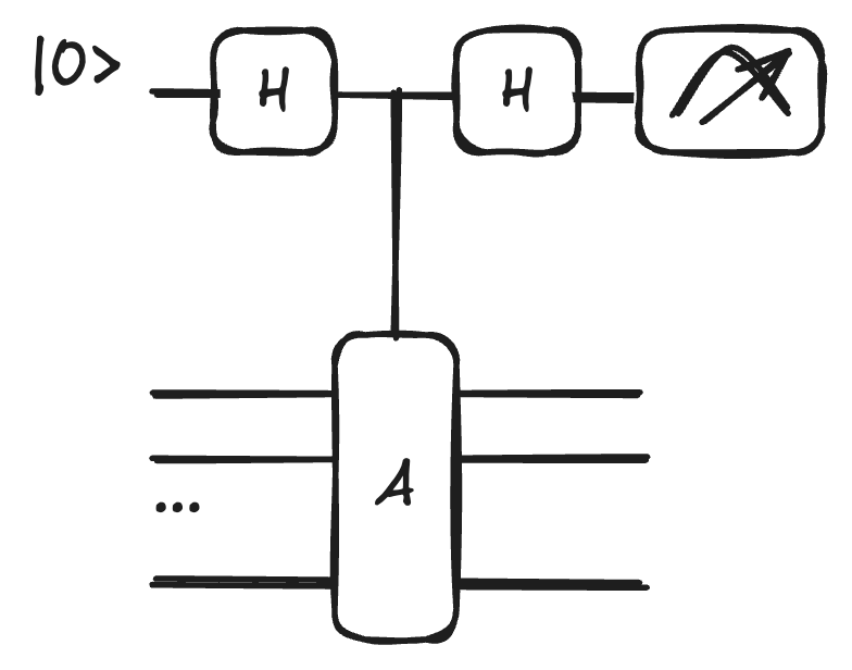
The joint state of the ancilla and the data $| ψ ⟩$ evolves as follows:

| 0 ⟩ \otimes | ψ ⟩ \overset{H}{\to} \frac{1}{\sqrt{2}} (| 0 ⟩ + | 1 ⟩) \otimes | ψ ⟩ \overset{Ctrl- A}{\to} \frac{1}{\sqrt{2}} (| 0 ⟩ | ψ ⟩ + | 1 ⟩ A | ψ ⟩)

Applying the second Hadamard yields:

\frac{1}{\sqrt{2}} (\frac{| 0 ⟩ + | 1 ⟩}{\sqrt{2}} | ψ ⟩ + \frac{| 0 ⟩ - | 1 ⟩}{\sqrt{2}} A | ψ ⟩) = | 0 ⟩ \otimes \frac{(I + A) | ψ ⟩}{2} + | 1 ⟩ \otimes \frac{(I - A) | ψ ⟩}{2}

Measuring the ancilla in the $| 0 ⟩$ state effectively applies the projection operator $P_{+} = \frac{1}{2} (I + A)$ , which projects the data onto the $+ 1$ eigenspace of $A$ .
If the state was already a $+ 1$ eigenstate, we simply get $| ψ ⟩$ back.

Exercise 14: Stabilizer Measurement Circuit

Suppose $| ψ ⟩$ is a $+ 1$ eigenstate of $A$ : $A | ψ ⟩ = + | ψ ⟩$ .
Trace through the circuit above and show that the ancilla measurement always returns $0$ .
Now suppose an error has occurred and $| ψ^{'} ⟩$ is a $- 1$ eigenstate: $A | ψ^{'} ⟩ = - | ψ^{'} ⟩$ .
Show that the ancilla measurement always returns $1$ .
In the case of the 3-qubit code with $A = Z_{1} Z_{2}$ , what specific gates replace the "controlled- $A$ " box?

Answer

If $A | ψ ⟩ = + | ψ ⟩$ , then after the controlled- $A$ :
$\frac{1}{\sqrt{2}} (| 0 ⟩ | ψ ⟩ + | 1 ⟩ | ψ ⟩) = \frac{1}{\sqrt{2}} (| 0 ⟩ + | 1 ⟩) | ψ ⟩$
After the second Hadamard: $| 0 ⟩ | ψ ⟩$ . Measurement always gives $0$ .
If $A | ψ^{'} ⟩ = - | ψ^{'} ⟩$ , then after the controlled- $A$ :
$\frac{1}{\sqrt{2}} (| 0 ⟩ | ψ^{'} ⟩ + | 1 ⟩ (- | ψ^{'} ⟩)) = \frac{1}{\sqrt{2}} (| 0 ⟩ - | 1 ⟩) | ψ^{'} ⟩$
After the second Hadamard: $| 1 ⟩ | ψ^{'} ⟩$ . Measurement always gives $1$ .
The controlled- $Z_{1} Z_{2}$ can be decomposed as two controlled- $Z$ gates (or equivalently, two CNOT gates from data qubits to the ancilla, since CNOT implements a controlled- $X$ which, combined with Hadamards on the ancilla, effectively measures $Z$ ).
In practice, for $Z$ -type stabilizers, we skip the Hadamards on the ancilla and just use two CNOTs from data qubits 1 and 2 to the ancilla.

Detectors and Decoding

Now that we have seen the full circuit of stabilizer measurements via repeated syndrome extraction, what should we do with all the ancilla bitstring?
How to recover the potentially corrupted encoded data state?
Before taking the example of the surface code, we discuss the decoding part by revisiting the repetition code with a focus on detectors and decoding.

The Logic of Sequential Measurements

In the bit-flip repetition code, we are interested in repeated parity $Z Z$ measurements.
As we already mentioned, we don't measure the state of the data qubits directly, as this would collapse the superposition we are trying to protect, but rather the relative parity between neighbors.

When we look at the results of these measurements, we are looking for consistency.
If we have a sequence of measurements, any change in the parity result over time or space signals that an error has occurred.
We define a Detector as a specific set of measurements that, in the absence of any errors, has a deterministic expected parity (usually even).

Detector Event

A Detector Event occurs when a detector returns an "unexpected parity."
It signals that an error has entered the system.
Crucially, a single measurement result in isolation tells us nothing; it is only the relationship between sequential measurements that allows us to track errors.

The intuition is that every sequential pair of measurements forms a detector.
It isn't the specific value of the individual measurement that carries the information, but rather the change between them.
For instance, if a measurement $m_{i}$ at time $t$ gives $0$ and the measurement at $t + 1$ gives $1$ , we know that an error must have occurred in the interval between those two measurements, because of this parity change.
In practice, here is an example a raw ancilla measurement sequence and its associated detection signal:

Ancilla Measurement Sequence	Detection Signal
$0 \to 0 \to 1 \to 1 \to 0$	$0 \to 1 \to 0 \to 1$
$0 \to 0 \to 0 \to 1 \to 1$	$0 \to 0 \to 1 \to 0$

The detection signal is essentially the XOR of consecutive bits.
A "1" in the detection signal indicates a detector event, a change in parity.
This is the first step toward building a "syndrome" that we can use for decoding.

The Error Detection Graph

To make sense of these detector events across many qubits (space) and many rounds of measurement (time), we map the problem onto a Spacetime Graph.
In this representation, we can visualize how physical errors (the "causes") manifest as detector events (the "symptoms").

Nodes represent potential detector events (the comparison between two measurements).
Edges represent the physical errors that "link" two detector events together.

An edge connects two nodes if a single physical error triggers exactly those two detector events.
For example, a bit-flip on a data qubit between two measurement rounds will only trigger the detectors that share that qubit, since after this bit-flip, future detectors will not see any new change.
A measurement error on an ancilla, however, might only trigger a "timelike" edge between two consecutive rounds of measurement at the same location.
An example of such a detection graphs is shown in Fig..

Spacetime detection graph for the repetition code. Nodes are detector events, horizontal edges are data errors, vertical edges are measurement errors, diagonal edges are data errors between CNOTs.|600 — **Spacetime detection graph for the repetition code.** Nodes are detector events, horizontal edges are data errors, vertical edges are measurement errors, diagonal edges are data errors between CNOTs.

Inferring Errors through Matching

When we actually run an experiment, we obtain a pattern of measurement results.
We then identify the nodes where the parity was unexpected.
Our goal is to find the most likely set of physical errors (edges) that could have produced this specific pattern of nodes.

This is fundamentally a graph problem.
If we see only two detector events, we can "match" them easily with an edge.
If we have a complex web of events, we use algorithms like Minimum Weight Perfect Matching (MWPM) to infer the most probable error chain.
This mapping of quantum errors to graphs is what makes error correction scalable 7.

Exercise 15: Detection Graph Analysis

Consider a distance- $3$ repetition code (3 data qubits, 2 ancillas) measured for 4 rounds.
The detection signal for ancilla 1 (measuring $Z_{1} Z_{2}$ ) is: $0, 1, 1, 0$ .
The detection signal for ancilla 2 (measuring $Z_{2} Z_{3}$ ) is: $0, 1, 1, 0$ .

At which time step did the detector events occur for each ancilla?
Is this pattern consistent with a single data error? If so, on which qubit and at what time?
Is this pattern also consistent with two measurement errors? Explain.

Answer

Detector events (where the detection signal = 1):
- Ancilla 1: events at times $t = 2$ and $t = 3$ (XOR flipped between rounds 1-2 and 2-3).
- Ancilla 2: events at times $t = 2$ and $t = 3$ .
Detection signal $0, 1, 1, 0$ means: no change between rounds 0-1, change between 1-2, change between 2-3, no change between 3-4.
This is consistent with a data error on qubit 2 occurring between rounds 1 and 2 (first detection at round 2), followed by another event between rounds 2 and 3.
Yes. Two measurement errors, one at round 2 and one at round 3 for both ancillas, could produce the same pattern.
This ambiguity is why MWPM decoding is needed: it finds the most probable explanation given the error rates.

Now that we are familiar with the stabilizer formalism and the decoding problem and having built intuition from the repetition code, we discuss the surface code, probably the most well studied QEC code.

Surface Code

Limitations of the Shor Code

The Shor Code showed we could protect against both $X$ and $Z$ errors by nesting codes.
However, the Shor code has a distinct hierarchy: we have local $Z$ checks to catch bit-flips, but the $X$ checks are "global" across blocks.

The disadvantage is the "non-locality" of the $X$ stabilizers.
In a physical architecture, requiring a 6-qubit joint measurement ( $X_{1} X_{2} X_{3} X_{4} X_{5} X_{6}$ ) is hardware-intensive and prone to introducing more errors than it fixes.

The Surface Code

The Surface Code takes a different approach.
Instead of mixing local and global checks, we make everything local.
By arranging qubits on a 2D lattice, we can perform all parity checks using only nearest-neighbor interactions involving 4 data qubits.

Key Concept: Local Parity

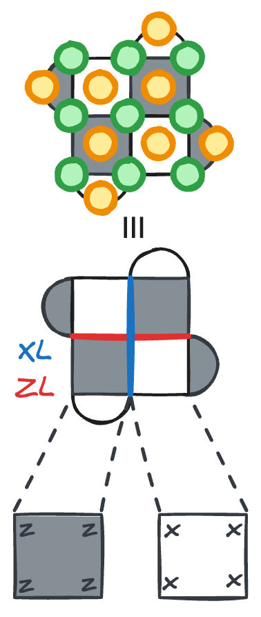
In the surface code, we define two types of plaquettes:

$Z$ -plaquettes (darker regions) which measure the parity of $Z$ operators on 4 surrounding data qubits to detect $X$ errors.
$X$ -plaquettes (lighter regions) which measure the parity of $X$ operators on 4 surrounding data qubits to detect $Z$ errors.

The logical codespace ( $Span {{| 0 ⟩}_{L}, {| 1 ⟩}_{L}}$ ) is defined as the $+ 1$ simultaneous eigenspace of all stabilizers.

The lattice structure is illustrated in Fig..

The surface code lattice: data qubits (green) sit on vertices, ancilla qubits (orange) are in the centers of (dark) and (light) tiles of the surface. Boundary-to-boundary product of physical operators define the logical operators (red) and blue.|300 — **The surface code lattice**: data qubits (green) sit on vertices, ancilla qubits (orange) are in the centers of $Z$ (dark) and $X$ (light) tiles of the surface. Boundary-to-boundary product of physical operators define the logical operators $Z_{L}$ (red) and ${| X ⟩}_{L}$ blue.

Intuition: Why Locality Matters

Locality means each stabilizer measurement only involves nearest-neighbor qubits on a 2D layout.
Long-range interactions are either impossible (superconducting chip) or error-prone (atom movement) on most platforms, so this matters a lot in practice.
The surface code gives the same protection as the Shor code but with only local operations, which is why it is the leading candidate for fault-tolerant quantum computing as the numerous experimental implementations show.

Surface code features

The 2D layout and the small weight of the stabilizers are the reasons why the surface code has been well studied.
Another reason that we will discuss soon is its high accuracy threshold: we can tolerate a lot of physical error probability per physical gate before the QEC protection stops working.

Constructing the Logical State

How to write the ${| 0 ⟩}_{L}$ of this code?
We will see that it is not as straightforward as the ${| 0 ⟩}_{L} = | 000 ⟩$ of the repetition code.
To construct the logical ${| 0 ⟩}_{L}$ , we start from a "vacuum" of physical $| 0 ⟩$ states and "project" them consecutively into the stabilizer subspace.
If we start from $| 0 \dots 0 ⟩$ and apply a stabilizer projector $P = \frac{1}{2} (I + X_{a})$ for each $X$ -type stabilizer, we create the necessary entanglement.
Each projector creates a superposition:

| 0 \dots 0 ⟩ + (- 1)^{a} | 0 \dots 1111 \dots 0 ⟩

where $a$ represents the measurement outcome.

As we apply successive stabilizer projectors, the state branches further (twice for each stabilizer), spreading entanglement across the surface.
The resulting state is a highly entangled superposition:

\begin{matrix} | 0_{L} ⟩ & = | 000000000 ⟩ + (- 1)^{d} | 000000110 ⟩ \\ + (- 1)^{a} | 011000000 ⟩ + (- 1)^{a + d} | 011000110 ⟩ \\ + (- 1)^{b} | 110110000 ⟩ + (- 1)^{b + d} | 110110110 ⟩ \\ + (- 1)^{a + b} | 101110000 ⟩ + (- 1)^{a + b + d} | 101110110 ⟩ \\ + (- 1)^{c} | 000011011 ⟩ + (- 1)^{c + d} | 000011101 ⟩ \\ + (- 1)^{a + c} | 011011011 ⟩ + (- 1)^{a + c + d} | 011011101 ⟩ \\ + (- 1)^{b + c} | 110101011 ⟩ + (- 1)^{b + c + d} | 110101101 ⟩ \\ + (- 1)^{a + b + c} | 101101011 ⟩ + (- 1)^{a + b + c + d} | 101101101 ⟩ \end{matrix}

Where $a, \dots, d$ represent the values of each $X$ plaquette measurement.

The Efficiency of the Stabilizer Formalism

When we look at a lattice of $N$ plaquettes, describing the state of the system by tracking every individual term in the Hilbert space becomes quickly unreasonable, as we are dealing with $2^{N}$ terms.
The stabilizer formalism avoids this entirely.
Instead of an exponential description of the state, we rely on a linear description via the stabilizers.
This is what makes such codes tractable despite the exponential size of the many-body Hilbert space.

Defining the Logical Operators

To actually use our code for computation, we need to define our logical space.
Since we are dealing with a stabilizer code, we will not define the code from its logical states ${| 0 ⟩}_{L}$ and ${| 1 ⟩}_{L}$ (we tried) but from the logical qubit Pauli operators.
Specifically, we want to find a logical $X_{L}$ operator.
From a physical perspective, $X_{L}$ is a string of physical $X$ operators stretching across the lattice, see Fig..
It cannot be just any string; it must commute with all the stabilizers in our stabilizer group $S$ .

Why Commutation Matters

Stabilizers are "blind" to the full codespace.
If a stabilizer measurement could distinguish between states within the codespace, it would necessarily collapse the logical state.
Therefore, any logical operator, which by definition moves us from one point in the codespace to another, must commute with all stabilizers to ensure it doesn't leave the "protected" subspace or trigger an error syndrome.

Any chain of physical $X$ operators connecting the top boundary to the bottom boundary is a valid logical $X_{L}$ , provided it commutes with the stabilizers.
These different "versions" of $X_{L}$ are actually equivalent up to a stabilizer (they are in the same homology class).

Logical $Z$ and the Geometry of Errors

Similarly, we define the logical $Z_{L}$ as a string of physical $Z$ operators connecting the left boundary to the right boundary.
For example, in a small lattice:

Z_{L} {| 1 ⟩}_{L} = Z_{3} Z_{4} Z_{5} {| 1 ⟩}_{L}

Geometric Intuition

Just as physical $X$ and $Z$ anti-commute when they act on the same qubit, logical $X_{L}$ and $Z_{L}$ anti-commute because their paths on the lattice cross an odd number of times.
This topological "intersection number" is the deep reason why the code works as a single logical unit.
The code distance $d$ equals the minimum length of such a logical operator string, which is why a larger lattice provides more protection.

In this picture, quantum information is not stored at specific locations but in the global, non-local properties of the entire lattice 8.

Exercise 16: Surface Code Logical Operators

Consider a distance- $3$ surface code on a $3 \times 3$ lattice of data qubits (with appropriate boundary conditions).

How many data qubits, $X$ -stabilizers, and $Z$ -stabilizers does the code have?
Verify the $[[n, k, d ∥ n, k, d]]$ parameters using $k = n - (number of stabilizers)$ .
Give an example of a weight-3 logical $X_{L}$ operator (a string of 3 $X$ operators crossing the lattice).
Why can't a weight-2 string of $X$ operators be a logical operator?

Answer

A distance-3 surface code has $n = d^{2} = 9$ data qubits (on a rotated lattice), 4 $X$ -stabilizers, and 4 $Z$ -stabilizers, for a total of 8 stabilizers.
$k = n - (stabilizers) = 9 - 8 = 1$ logical qubit. $d = 3$ .
So the code is $[[9, 1, 3 ∥ 9, 1, 3]]$ .
A horizontal string of $X_{1} X_{2} X_{3}$ along one column of the lattice (connecting top boundary to bottom boundary if $X_{L}$ runs vertically in your convention).
A weight-2 string would not span the full lattice.
It would either be equivalent to a stabilizer (if it forms a closed loop) or anti-commute with some stabilizer (if it's a partial string).
Neither case gives a valid logical operator.

The Threshold Theorem and Scaling

We briefly mentioned the high accuracy threshold of the surface code as being one of the nice features of this code.
Now it's time to be more precise on this specific point.

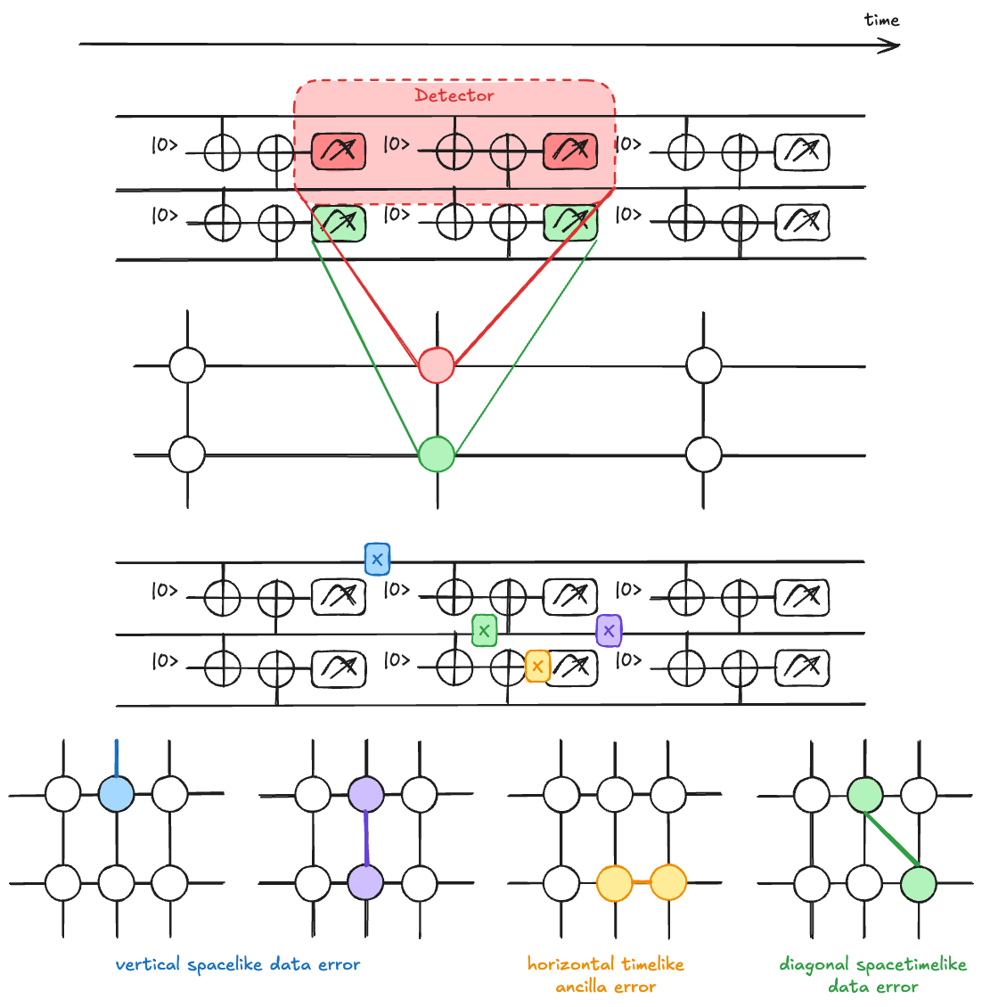
Classes of Errors

First, when we analyze how errors propagate and are caught in a QEC code like the surface code, we saw that we categorize them based on their orientation in the (2+1)D spacetime volume (the "+1" standing for time), just as we did above in the Decoding part:

Horizontal matching corresponds to time-like errors: syndrome measurement failures. A flip in the measurement outcome appears as two syndrome changes separated in time.
Vertical matching represents space-like errors: the "classic" data qubit errors (Pauli $X$ or $Z$ ) that occur on the physical qubits between measurement cycles.
Diagonal matching represents spacetime errors: often arising from errors during the entangling gates (like a CNOT) of the stabilizer measurement circuit itself. A single failure in a CNOT can propagate to both the data qubit and the ancilla, creating a correlated error that is diagonal in our decoding graph.

The Threshold

To visualize if our error correction is actually helping, we use a Threshold Plot.
This plot compares the physical error rate $p$ against the logical error rate $P_{L}$ .

As we increase the code distance $d$ , we see a distinct behavior change at a specific point called the threshold $p_{th}$ .

We can model the logical error rate as:

P_{L} \approx C \cdot {(\frac{p}{p_{th}})}^{\frac{d + 1}{2}}

When $p < p_{th}$ : We are in the "protection" regime. More is better. Increasing the distance $d$ suppresses the logical error rate exponentially.
When $p > p_{th}$ : We are in the "noise-dominated" regime. More is worse. Adding more qubits just adds more opportunities for errors to occur, and the complex decoding can no longer keep up. The logical error rate actually increases with $d$ , eventually saturating at $P_{L} = 50 %$ , which represents total loss of information (random noise).

This behavior is shown in the threshold plot Fig..

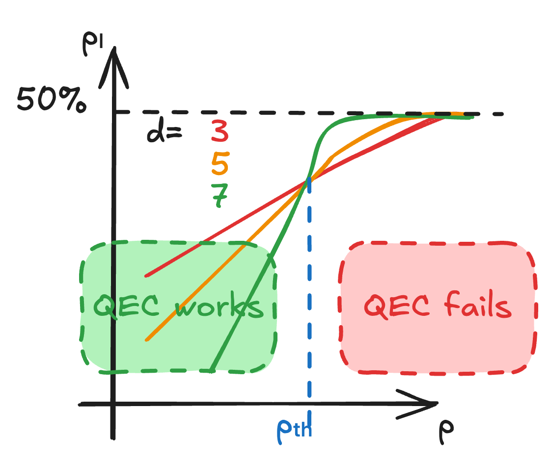
Threshold plot: logical error rate vs physical error rate for different code distances (red), (orange) and (green). The curves cross at the threshold , (dashed blue line).|400 — Threshold plot: logical error rate $P_{L}$ vs physical error rate $p$ for different code distances $d = 3$ (red), $5$ (orange) and $7$ (green). The curves cross at the threshold $p_{th}$ , (dashed blue line).

Key Takeaway

The abscisse of the "crossing point" on the graph is the threshold $p_{th}$ .
For the surface code under circuit-level noise, this is often cited around $1 %$ 7.
But be aware that this value varies significantly depending on the noise model of the gates, the circuit implementation and the decoder used.
Current superconducting and neutral atom platforms are operating near or just below this threshold.

Exercise 17: Threshold Calculation

Using the approximate formula $P_{L} \approx 0.1 \cdot (p / p_{th})^{(d + 1) / 2}$ with $p_{th} = 1 %$ :

For $p = 0.1 %$ and $d = 3$ , compute $P_{L}$ .
For $p = 0.1 %$ and $d = 5$ , compute $P_{L}$ .
For $p = 0.1 %$ and $d = 7$ , compute $P_{L}$ .
By what factor does $P_{L}$ decrease when going from $d = 3$ to $d = 5$ ? What about $d = 5$ to $d = 7$ ?

Answer

With $p / p_{th} = 0.001 / 0.01 = 0.1$ :

$P_{L} = 0.1 \cdot (0.1)^{(3 + 1) / 2} = 0.1 \cdot (0.1)^{2} = 0.1 \cdot 0.01 = 10^{- 3}$
$P_{L} = 0.1 \cdot (0.1)^{(5 + 1) / 2} = 0.1 \cdot (0.1)^{3} = 0.1 \cdot 10^{- 3} = 10^{- 4}$
$P_{L} = 0.1 \cdot (0.1)^{(7 + 1) / 2} = 0.1 \cdot (0.1)^{4} = 0.1 \cdot 10^{- 4} = 10^{- 5}$
From $d = 3$ to $d = 5$ : factor of $10^{- 3} / 10^{- 4} = 10$ improvement.
From $d = 5$ to $d = 7$ : factor of $10^{- 4} / 10^{- 5} = 10$ improvement.
Each increment of 2 in distance gives another order of magnitude in error suppression (when $p / p_{th} = 0.1$ ).

Circuit Implementation and Fault-Tolerant Design

When we move from the theoretical framework of the surface code to its physical implementation, we must consider the specific gates that realize our stabilizers.
A $Z$ -plaquette corresponds to a $Z Z Z Z$ operator acting on four data qubits, which detects $X$ errors.
An $X$ -stabilizer corresponds to an $X X X X$ operator designed to detect $Z$ errors.

To measure these stabilizers without destroying the quantum information in the data qubits, we introduce an ancilla qubit, just like for the repetition code.
The circuit involves a sequence of four CNOT gates (compared to 2 for the repetition code) between the ancilla and the data qubits.
But we cannot apply these gates in any arbitrary order.
The sequence of CNOTs matters for fault tolerance because of how errors propagate through the circuit.

The Intuition of Error Propagation

Again, our goal is to detect errors in the data by periodically checking the stabilizers via the ancilla.
But the ancilla itself is a physical qubit prone to noise.
If a single error occurs on the ancilla during the measurement sequence and propagates to multiple data qubits, we risk creating a high-weight error from a single fault.

Consider the "Hook error."
If a single $X$ error occurs on the ancilla qubit halfway through the measurement of a $Z$ -stabilizer, it can propagate to the remaining data qubits in the sequence.
In a four-qubit plaquette, an error after the second CNOT could result in a $Z Z$ error on the data.

Hook Errors

A single fault on an ancilla that propagates to two or more data qubits is often called a hook error.
In the surface code, if these errors align poorly, they can effectively reduce the code distance.

Gate Ordering

The danger arises when propagated errors align with our logical operators.
For a distance-3 surface code, one hook error could lead to 2 physical data errors, hence a logical one.
On a distance-5 code, if two hook errors occur due to unlucky CNOT ordering, they could lead to 4 data errors that form a chain across the lattice, potentially also resulting in a logical error.

To prevent this, we follow a specific design rule: the last two qubits touched by a $Z$ -stabilizer measurement must propagate errors perpendicular to the logical $Z_{L}$ operator.
By orienting the "stretch" of the hook error so it doesn't bridge the gap between boundaries, we ensure that the error weight remains manageable (aka does not increase) and doesn't lead to a premature logical failure.

One solution is to use a specific CNOT ordering, often a "Z-shape" or "N-shape" on qubits in the plaquette.
Specific orderings ensure that the "last 2 qubits touched" rule is preserved, as shown in Fig..

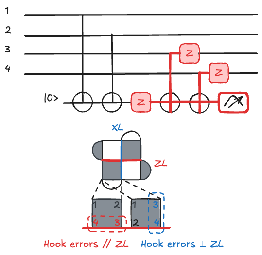
Comparison of CNOT ordering for a Z stabilizer to ensure fault tolerance.|600 — Comparison of CNOT ordering for a Z stabilizer to ensure fault tolerance.

Note

This specific geometric solution for gate ordering is not unique, but it is mandatory for maintaining the threshold of the surface code.
The specific mapping differs for architectures like Neutral Atoms due to different connectivity and constraints.

Exercise 18: Hook Error Analysis

Consider a $Z$ -plaquette measuring $Z_{1} Z_{2} Z_{3} Z_{4}$ with the CNOT sequence: ancilla controls qubits in a circle order.

If an $X$ error occurs on the ancilla between the 2nd and 3rd CNOT, which data qubits are affected? What is the resulting data error?
If instead the CNOT order is 1, 3, 2, 4, and the same $X$ error occurs between the 2nd and 3rd CNOT, which data qubits are affected?
Explain why the second ordering is better for fault tolerance in the surface code.

Answer

With ordering 1, 2, 3, 4: the $X$ error after the 2nd CNOT propagates via the 3rd and 4th CNOTs.
Each CNOT (ancilla as control for $Z$ measurement) propagates $X$ errors from ancilla to data.
The data qubits 3 and 4 receive $Z$ errors (via the CNOT propagation rule).
Resulting error: $Z_{3} Z_{4}$ on the data, a weight-2 error.
With ordering 1, 3, 2, 4: after the 2nd CNOT (which targets qubit 3), the $X$ error propagates via the 3rd CNOT (targeting qubit 2) and 4th CNOT (targeting qubit 4).
Resulting error: $Z_{2} Z_{4}$ on the data.
In the surface code, qubits 3 and 4 in ordering (a) are adjacent and their $Z_{3} Z_{4}$ error aligns with the logical $Z_{L}$ string direction, potentially bridging boundaries.
In ordering (b), $Z_{2} Z_{4}$ are not adjacent along the logical string direction; they stretch perpendicular to $Z_{L}$ .
A perpendicular error is less dangerous because it doesn't contribute to shortening the effective code distance along the logical operator direction.

The Surface Code Detection Graph

To decode errors on the Surface code, we move from a 2D physical layout to a 3D Detection Graph.
While a 1D repetition code allows us to visualize errors on a line, the surface code requires a 2D plane of qubits.
When we add the dimension of time (the repeated measurement rounds), we get a 3D spacetime volume.

Nothing differs from the repetition code: in this graph, "nodes" still represent stabilizer measurement events, and "edges" represent potential errors (either physical qubit flips or measurement bit-flips).
If a stabilizer changes its value between round $t$ and $t + 1$ , it "triggers," creating a defect in the graph.
The job of the decoder is then to pair these defects in a way that most likely explains the underlying physical noise.

Implementing Logical Gates

Logical Initialization and Measurement

We briefly mention two important logical operations: initialization and measurement.
We begin with logical initialization, where we prepare the code in a specific state.
For the surface code, we typically initialize the logical state ${| 0 ⟩}_{L}$ by preparing all physical data qubits in the $| 0 ⟩$ state and measuring the $X$ stabilizers once.
Indeed, projecting (via measuring) the $X$ -type stabilizers is what "adds" the missing constraints and creates the entanglement of the encoded ${| 0 ⟩}_{L}$ .
Conversely, to prepare the logical ${| + ⟩}_{L}$ state, we initialize all physical qubits in the $| + ⟩$ basis and measure the $Z$ stabilizers.

Logical measurement in the $Z_{L}$ basis is performed by measuring all physical data qubits in the $Z$ basis ( $M_{z}$ ).
We then aggregate these results to determine the parity of the logical operator.
Similarly, measurement in the $X_{L}$ basis involves measuring all physical data qubits in the $X$ basis ( $M_{x}$ ).

The Surface Code Memory Experiment

The "Memory Experiment" is the basic test of whether a quantum error-correcting code actually works, relying simply on logical initialization, repeated stabilizer measurement and logical measurement.
The goal is simple: can we keep a logical qubit alive longer than its constituent physical parts?

The procedure follows a specific cadence.
First, we initialize the logical state ${| 0 ⟩}_{L}$ .
Then, we enter a "syndrome extraction" phase consisting of repeated rounds of stabilizer measurements.
In each round, we measure the parity of $X$ -type and $Z$ -type stabilizers to detect if any Pauli errors have occurred.

Stabilization Rounds

We don't just measure once.
Because our measurements themselves are noisy, we must repeat these rounds $d$ times (where $d$ is the code distance) to build up enough temporal confidence to distinguish between a real qubit error and a faulty measurement outcome.

Finally, we perform a logical $Z_{L}$ measurement.
By comparing the initial state, the history of measurement syndromes, and the final readout, we can determine if the logical information remained intact.

Storing a logical qubit via a memory experiment is not enough though, we also need to manipulate it.
Some manipulations are easier than others: for the surface code, the logical CNOT and the Hadamard are transversal (modulo some hidden details), it means that a logical gate is applied by simply performing the same gate on every physical qubit.
However, the Eastin-Knill theorem tells us that no single code can implement a universal gate set transversally.
How to get a non-Clifford gate then?
We rely on quantum teleportation.

Non-Clifford Gates: T via Teleportation

The most difficult gate to implement fault-tolerantly is the $T$ gate ( $T = diag (1, e^{i π / 4})$ ), which is essential for universality.
Since we cannot perform it transversally on the surface code without destroying the code's protection, we use Gate Teleportation.

The idea is to "pre-bake" the non-Cliffordness into a special resource state, called a Magic State $| ϕ ⟩ = T | + ⟩$ .
We then use only Clifford operations (which are "easy" and fault-tolerant) to consume this magic state and teleport the $T$ gate onto our target logical state $| ψ ⟩$ .

The circuit logic backpropagate a $T$ gate into a classic teleportation circuit, following the relation $T X T^{†} = e^{- i π / 4} S X$ .
If we measure the resource qubit and get a "1" outcome, we must apply a corrective $S$ gate (an "Easy" Clifford) to finish the operation.

| ϕ ⟩ = T | + ⟩ = \frac{| 0 ⟩ + e^{i π / 4} | 1 ⟩}{\sqrt{2}}

Then, the process of Magic State Distillation allows us to convert many of such noisy non-Clifford states into one highly pure state, which we then inject into our computation using the circuit shown in Fig..

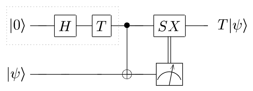
Circuit diagram for T-gate teleportation using a magic state and a corrective S gate.|600 — Circuit diagram for T-gate teleportation using a magic state and a corrective S gate.

Exercise 19: Magic State Properties

The magic state is $| T ⟩ = T | + ⟩ = \frac{1}{\sqrt{2}} (| 0 ⟩ + e^{i π / 4} | 1 ⟩)$ .

Show that $| T ⟩$ is not a stabilizer state (i.e., it cannot be the $+ 1$ eigenstate of any single Pauli operator).
Compute $⟨ T | X | T ⟩$ , $⟨ T | Y | T ⟩$ , and $⟨ T | Z | T ⟩$ . Where does $| T ⟩$ sit on the Bloch sphere?
Why is it significant that the $T$ gate cannot be implemented transversally? What does the Eastin-Knill theorem say?

Answer

A stabilizer state must lie on an axis of the Bloch sphere ( $\pm x$ , $\pm y$ , or $\pm z$ ).
$| T ⟩$ has a phase of $π / 4$ on the $| 1 ⟩$ component, placing it at a $45^{\circ}$ angle between the $x$ and $y$ axes on the equator.
It is not an eigenstate of $X$ , $Y$ , or $Z$ , so it is not a stabilizer state.
$⟨ T | X | T ⟩ = \frac{1}{2} (⟨ 0 | + e^{- i π / 4} ⟨ 1 |) (X) (| 0 ⟩ + e^{i π / 4} | 1 ⟩)$
$= \frac{1}{2} (⟨ 0 | + e^{- i π / 4} ⟨ 1 |) (| 1 ⟩ + e^{i π / 4} | 0 ⟩)$
$= \frac{1}{2} (e^{i π / 4} + e^{- i π / 4}) = \cos (π / 4) = 1 / \sqrt{2}$ .
Similarly $⟨ T | Y | T ⟩ = 1 / \sqrt{2}$ and $⟨ T | Z | T ⟩ = 0$ .
The state sits on the equator of the Bloch sphere at angle $π / 4$ between the $+ x$ and $+ y$ axes.
The Eastin-Knill theorem states that no quantum error-correcting code can implement a universal gate set entirely through transversal gates.
Since Clifford gates alone are not universal (they can be efficiently classically simulated by the Gottesman-Knill theorem), we need at least one non-Clifford gate ( $T$ ) for universality.
The $T$ gate must therefore be implemented via non-transversal methods like magic state injection and distillation.

Exercise 20: Resource Overhead for the Surface Code

A distance- $d$ surface code uses approximately $2 d^{2} - 1$ physical qubits (data + ancilla) to encode 1 logical qubit.

How many physical qubits are needed for $d = 3, 5, 7, 9, 11$ ?
If we need a logical error rate of $P_{L} = 10^{- 15}$ (required for useful quantum computation), and the physical error rate is $p = 10^{- 3}$ with threshold $p_{th} = 10^{- 2}$ , estimate the required distance $d$ using $P_{L} \approx 0.1 \cdot (p / p_{th})^{(d + 1) / 2}$ .
How many physical qubits does this require for a single logical qubit? For 100 logical qubits?

Answer

Physical qubits
- $d = 3$ : $2 (9) - 1 = 17$ qubits
- $d = 5$ : $2 (25) - 1 = 49$ qubits
- $d = 7$ : $2 (49) - 1 = 97$ qubits
- $d = 9$ : $2 (81) - 1 = 161$ qubits
- $d = 11$ : $2 (121) - 1 = 241$ qubits
We need $0.1 \cdot (0.1)^{(d + 1) / 2} \leq 10^{- 15}$ .
$(0.1)^{(d + 1) / 2} \leq 10^{- 14}$ , so $(d + 1) / 2 \geq 14$ , giving $d \geq 27$ .
We need $d = 27$ (rounding to the nearest odd number).
For $d = 27$ : $2 (27^{2}) - 1 = 2 (729) - 1 = 1457$ physical qubits per logical qubit.
For 100 logical qubits: $100 \times 1457 = 145,700$ physical qubits.
This does not include the overhead for magic state distillation factories, which can increase the total by a lot.

Experimental Implementations of QEC

We end these lecture notes by some "preview material" that we will be covered in detail during next week's lecture, connecting the theoretical framework above to the state of experimental QEC.
It is based on the review 9 and the associated database accessible at github.com/francois-marie/awesome-quantum-computing-experiments.

Platforms and Codes

Experimental efforts have explored a variety of QEC codes across multiple hardware platforms.
The platforms considered include:

Superconducting Circuits (Transmons, Fluxoniums) 10
Trapped Ions 11
Neutral Atoms (in optical tweezers) 12
Photonic Systems (linear optics, integrated photonics)
NV Centers in Diamond 13
Nuclear Magnetic Resonance (NMR, for historical reasons)

The codes implemented experimentally range from simple repetition codes to topological codes:

Repetition Codes (distance $d$ , $[[d, 1, d ∥ d, 1, d]]$ for bit-flip or phase-flip) 14, ?, ?
Four-qubit codes ( $[[4, 1, 2 ∥ 4, 1, 2]]$ or $[[4, 2, 2 ∥ 4, 2, 2]]$ ) 15, ?
$[[5, 1, 3 ∥ 5, 1, 3]]$ Perfect Code 16
Steane $[[7, 1, 3 ∥ 7, 1, 3]]$ Code
Surface Codes (various distances) 17, ?, ?
Color Codes 18, ?
Bacon-Shor Codes 19

Timeline

The field has progressed through several milestones:

First QEC demonstrations (1998-2011): Early NMR and trapped ion experiments demonstrated basic 3-qubit codes 14, ?, ?.
Scaling to larger codes (2014-2021): Superconducting circuits began demonstrating repeated error correction and exponential error suppression with code distance 20, ?.
Below-threshold operation (2022-2024): Google demonstrated that increasing code distance from $d = 3$ to $d = 5$ to $d = 7$ reduces logical error rates, crossing the break-even point 17, ?.
Logical processors (2024-present): Neutral atom platforms demonstrated 48 logical qubits with color codes 21, and superconducting platforms demonstrated logical computation 22.

Intuition: Where We Stand

Multiple platforms have now demonstrated below-threshold operation for the repetition code and small surface codes.
The next step is below-threshold operation for the full surface code at increasing distances, and performing useful logical computations with encoded qubits.
This requires improvements in qubit quality, qubit count, and real-time decoding speed.

We will discuss these experimental results in depth during next week's lecture.

Conclusion

We started this lecture by seeing that classical error correction protects information through redundancy and majority voting.
The Hamming code does this efficiently, with overhead growing only logarithmically.

In the quantum setting, two constraints change everything: the No-Cloning Theorem forbids copying unknown states, and measurement back-action means we cannot inspect qubits without disturbing them.
These constraints force us to use parity measurements and entanglement instead.

The 3-qubit repetition codes showed the central trick: measure parity rather than individual qubits just like for the Hamming code, and you can extract error information without collapsing the logical state.
The Shor code extended this to protect against all single-qubit errors simultaneously, and showed that continuous errors are effectively digitized by syndrome measurement.

The stabilizer formalism gave us a compact language to describe codes: instead of tracking exponentially many amplitudes, we track a linear number of operators.
This led to the surface code, where all stabilizers are local.

We discussed the threshold theorem (error correction works as long as physical error rates are below a critical value) and fault-tolerant circuit design (careful gate ordering prevents single faults from cascading into logical errors).
We also saw how logical gates are implemented, with Clifford gates being straightforward and the $T$ gate requiring magic state injection.

In essence, without quantum error correction, the algorithms from our previous lectures (Shor, Grover, QPE) remain theoretical.
QEC is what bridges the gap and connects the noisy physical qubits from our platform lectures to the logical qubits that algorithms need.
Next week, we look at how different platforms implement these codes in practice.

References

1.: Acharya, R; Abanin, D; Aghababaie-Beni, L; Aleiner, I; Andersen, T; Ansmann, M; Arute, F; Arya, K; Asfaw, A; Astrakhantsev, N; Atalaya, J; Babbush, R; Bacon, D; Ballard, B; Bardin, J; Bausch, J; Bengtsson, A; Bilmes, A; Blackwell, S; Boixo, S; Bortoli, G; Bourassa, A; Bovaird, J; Brill, L; Broughton, M; Browne, D; Buchea, B; Buckley, B; Buell, D; Burger, T; Burkett, B; Bushnell, N; Cabrera, A; Campero, J; Chang, H; Chen, Y; Chen, Z; Chiaro, B; Chik, D; Chou, C; Claes, J; Cleland, A; Cogan, J; Collins, R; Conner, P; Courtney, W; Crook, A; Curtin, B; Das, S; Davies, A; De Lorenzo, L; Debroy, D; Demura, S; Devoret, M; Di Paolo, A; Donohoe, P; Drozdov, I; Dunsworth, A; Earle, C; Edlich, T; Eickbusch, A; Elbag, A; Elzouka, M; Erickson, C; Faoro, L; Farhi, E; Ferreira, V; Burgos, L; Forati, E; Fowler, A; Foxen, B; Ganjam, S; Garcia, G; Gasca, R; Genois, É; Giang, W; Gidney, C; Gilboa, D; Gosula, R; Dau, A; Graumann, D; Greene, A; Gross, J; Habegger, S; Hall, J; Hamilton, M; Hansen, M; Harrigan, M; Harrington, S; Heras, F; Heslin, S; Heu, P; Higgott, O; Hill, G; Hilton, J; Holland, G; Hong, S; Huang, H; Huff, A; Huggins, W; Ioffe, L; Isakov, S; Iveland, J; Jeffrey, E; Jiang, Z; Jones, C; Jordan, S; Joshi, C; Juhas, P; Kafri, D; Kang, H; Karamlou, A; Kechedzhi, K; Kelly, J; Khaire, T; Khattar, T; Khezri, M; Kim, S; Klimov, P; Klots, A; Kobrin, B; Kohli, P; Korotkov, A; Kostritsa, F; Kothari, R; Kozlovskii, B; Kreikebaum, J; Kurilovich, V; Lacroix, N; Landhuis, D; Lange-Dei, T; Langley, B; Laptev, P; Lau, K; Le Guevel, L; Ledford, J; Lee, J; Lee, K; Lensky, Y; Leon, S; Lester, B; Li, W; Li, Y; Lill, A; Liu, W; Livingston, W; Locharla, A; Lucero, E; Lundahl, D; Lunt, A; Madhuk, S; Malone, F; Maloney, A; Mandrà, S; Manyika, J; Martin, L; Martin, O; Martin, S; Maxfield, C; McClean, J; McEwen, M; Meeks, S; Megrant, A; Mi, X; Miao, K; Mieszala, A; Molavi, R; Molina, S; Montazeri, S; Morvan, A; Movassagh, R; Mruczkiewicz, W; Naaman, O; Neeley, M; Neill, C; Nersisyan, A; Neven, H; Newman, M; Ng, J; Nguyen, A; Nguyen, M; Ni, C; Niu, M; O’Brien, T; Oliver, W; Opremcak, A; Ottosson, K; Petukhov, A; Pizzuto, A; Platt, J; Potter, R; Pritchard, O; Pryadko, L; Quintana, C; Ramachandran, G; Reagor, M; Redding, J; Rhodes, D; Roberts, G; Rosenberg, E; Rosenfeld, E; Roushan, P; Rubin, N; Saei, N; Sank, D; Sankaragomathi, K; Satzinger, K; Schurkus, H; Schuster, C; Senior, A; Shearn, M; Shorter, A; Shutty, N; Shvarts, V; Singh, S; Sivak, V; Skruzny, J; Small, S; Smelyanskiy, V; Smith, W; Somma, R; Springer, S; Sterling, G; Strain, D; Suchard, J; Szasz, A; Sztein, A; Thor, D; Torres, A; Torunbalci, M; Vaishnav, A; Vargas, J; Vdovichev, S; Vidal, G; Villalonga, B; Heidweiller, C; Waltman, S; Wang, S; Ware, B; Weber, K; Weidel, T; White, T; Wong, K; Woo, B; Xing, C; Yao, Z; Yeh, P; Ying, B; Yoo, J; Yosri, N; Young, G; Zalcman, A; Zhang, Y; Zhu, N; Zobrist, N . Quantum error correction below the surface code threshold. Nature 638 (8052) , 920–926 (2025) . doi:10.1038/s41586-024-08449-y
2.: Chen, Z; Satzinger, K; Atalaya, J; Korotkov, A; Dunsworth, A; Sank, D; Quintana, C; McEwen, M; Barends, R; Klimov, P; Hong, S; Jones, C; Petukhov, A; Kafri, D; Demura, S; Burkett, B; Gidney, C; Fowler, A; Paler, A; Putterman, H; Aleiner, I; Arute, F; Arya, K; Babbush, R; Bardin, J; Bengtsson, A; Bourassa, A; Broughton, M; Buckley, B; Buell, D; Bushnell, N; Chiaro, B; Collins, R; Courtney, W; Derk, A; Eppens, D; Erickson, C; Farhi, E; Foxen, B; Giustina, M; Greene, A; Gross, J; Harrigan, M; Harrington, S; Hilton, J; Ho, A; Huang, T; Huggins, W; Ioffe, L; Isakov, S; Jeffrey, E; Jiang, Z; Kechedzhi, K; Kim, S; Kitaev, A; Kostritsa, F; Landhuis, D; Laptev, P; Lucero, E; Martin, O; McClean, J; McCourt, T; Mi, X; Miao, K; Mohseni, M; Montazeri, S; Mruczkiewicz, W; Mutus, J; Naaman, O; Neeley, M; Neill, C; Newman, M; Niu, M; O’Brien, T; Opremcak, A; Ostby, E; Pató, B; Redd, N; Roushan, P; Rubin, N; Shvarts, V; Strain, D; Szalay, M; Trevithick, M; Villalonga, B; White, T; Yao, Z; Yeh, P; Yoo, J; Zalcman, A; Neven, H; Boixo, S; Smelyanskiy, V; Chen, Y; Megrant, A; Kelly, J . Exponential suppression of bit or phase errors with cyclic error correction. Nature 595 (7867) , 383–387 (2021) . doi:10.1038/s41586-021-03588-y
3.: Shor, P . Scheme for reducing decoherence in quantum computer memory. Physical Review A 52 (4) , R2493–R2496 (1995) . doi:10.1103/PhysRevA.52.R2493
4.: Nielsen, M; Chuang, I . Quantum Computation and Quantum Information 10th Anniversary Edition. (2000) . doi:10.1017/CBO9780511976667
5.: Terhal, B . Quantum Error Correction for Quantum Memories. Reviews of Modern Physics 87 (2) , 307–346 (2015) . doi:10.1103/RevModPhys.87.307
6.: Gottesman, D . Stabilizer Codes and Quantum Error Correction. (1997) . doi:10.7907/rzr7-dt72
7.: Fowler, A; Mariantoni, M; Martinis, J; Cleland, A . Surface codes: Towards practical large-scale quantum computation. (2012) . doi:10.48550/arXiv.1208.0928
8.: Kitaev, A . Fault-tolerant quantum computation by anyons. Annals of Physics 303 (1) , 2–30 (2003) . doi:https://doi.org/10.1016/S0003-4916(02)00018-0
9.: Le Régent, F . Awesome Quantum Computing Experiments: Benchmarking Experimental Progress Towards Fault-Tolerant Quantum Computation. (2025) . doi:10.48550/arXiv.2507.03678
10.: Kjaergaard, M; Schwartz, M; Braumüller, J; Krantz, P; Wang, J; Gustavsson, S; Oliver, W . Superconducting Qubits: Current State of Play. Annual Review of Condensed Matter Physics 11 (1) , 369–395 (2020) . doi:10.1146/annurev-conmatphys-031119-050605
11.: Bruzewicz, C; Chiaverini, J; McConnell, R; Sage, J . Trapped-Ion Quantum Computing: Progress and Challenges. Applied Physics Reviews 6 (2) , 021314 (2019) . doi:10.1063/1.5088164
12.: Wintersperger, K; Dommert, F; Ehmer, T; Hoursanov, A; Klepsch, J; Mauerer, W; Reuber, G; Strohm, T; Yin, M; Luber, S . Neutral Atom Quantum Computing Hardware: Performance and End-User Perspective. EPJ Quantum Technology 10 (1) , 32 (2023) . doi:10.1140/epjqt/s40507-023-00190-1
13.: Pezzagna, S; Meijer, J . Quantum computer based on color centers in diamond. Applied Physics Reviews 8 (1) , 011308 (2021) . doi:10.1063/5.0007444
14.: Cory, D; Price, M; Maas, W; Knill, E; Laflamme, R; Zurek, W; Havel, T; Somaroo, S . Experimental Quantum Error Correction. Phys. Rev. Lett. 81 (10) , 2152–2155 (1998) . doi:10.1103/PhysRevLett.81.2152
15.: Linke, N; Gutierrez, M; Landsman, K; Figgatt, C; Debnath, S; Brown, K; Monroe, C . Fault-tolerant quantum error detection. Science Advances 3 (10) , e1701074 (2017) . doi:10.1126/sciadv.1701074
16.: Knill, E; Laflamme, R; Martinez, R; Negrevergne, C . Implementation of the Five Qubit Error Correction Benchmark. Physical Review Letters 86 (25) , 5811–5814 (2001) . doi:10.1103/PhysRevLett.86.5811
17.: Acharya, R; Aleiner, I; Allen, R; Andersen, T; Ansmann, M; Arute, F; Arya, K; Asfaw, A; Atalaya, J; Babbush, R; Bacon, D; Bardin, J; Basso, J; Bengtsson, A; Boixo, S; Bortoli, G; Bourassa, A; Bovaird, J; Brill, L; Broughton, M; Buckley, B; Buell, D; Burger, T; Burkett, B; Bushnell, N; Chen, Y; Chen, Z; Chiaro, B; Cogan, J; Collins, R; Conner, P; Courtney, W; Crook, A; Curtin, B; Debroy, D; Barba, A; Demura, S; Dunsworth, A; Eppens, D; Erickson, C; Faoro, L; Farhi, E; Fatemi, R; Burgos, L; Forati, E; Fowler, A; Foxen, B; Giang, W; Gidney, C; Gilboa, D; Giustina, M; Dau, A; Gross, J; Habegger, S; Hamilton, M; Harrigan, M; Harrington, S; Higgott, O; Hilton, J; Hoffmann, M; Hong, S; Huang, T; Huff, A; Huggins, W; Ioffe, L; Isakov, S; Iveland, J; Jeffrey, E; Jiang, Z; Jones, C; Juhas, P; Kafri, D; Kechedzhi, K; Kelly, J; Khattar, T; Khezri, M; Kieferová, M; Kim, S; Kitaev, A; Klimov, P; Klots, A; Korotkov, A; Kostritsa, F; Kreikebaum, J; Landhuis, D; Laptev, P; Lau, K; Laws, L; Lee, J; Lee, K; Lester, B; Lill, A; Liu, W; Locharla, A; Lucero, E; Malone, F; Marshall, J; Martin, O; McClean, J; McCourt, T; McEwen, M; Megrant, A; Costa, B; Mi, X; Miao, K; Mohseni, M; Montazeri, S; Morvan, A; Mount, E; Mruczkiewicz, W; Naaman, O; Neeley, M; Neill, C; Nersisyan, A; Neven, H; Newman, M; Ng, J; Nguyen, A; Nguyen, M; Niu, M; O'Brien, T; Opremcak, A; Platt, J; Petukhov, A; Potter, R; Pryadko, L; Quintana, C; Roushan, P; Rubin, N; Saei, N; Sank, D; Sankaragomathi, K; Satzinger, K; Schurkus, H; Schuster, C; Shearn, M; Shorter, A; Shvarts, V; Skruzny, J; Smelyanskiy, V; Smith, W; Sterling, G; Strain, D; Szalay, M; Torres, A; Vidal, G; Villalonga, B; Heidweiller, C; White, T; Xing, C; Yao, Z; Yeh, P; Yoo, J; Young, G; Zalcman, A; Zhang, Y; Zhu, N . Suppressing quantum errors by scaling a surface code logical qubit. Nature 614 (7949) , 676–681 (2023) . doi:10.1038/s41586-022-05434-1
18.: Bluvstein, D; Levine, H; Semeghini, G; Wang, T; Ebadi, S; Kalinowski, M; Keesling, A; Maskara, N; Pichler, H; Greiner, M; Vuletić, V; Lukin, M . A quantum processor based on coherent transport of entangled atom arrays. Nature 604 (7906) , 451–456 (2022) . doi:10.1038/s41586-022-04592-6
19.: Egan, L; Debroy, D; Noel, C; Risinger, A; Zhu, D; Biswas, D; Newman, M; Li, M; Brown, K; Cetina, M; Monroe, C . Fault-tolerant control of an error-corrected qubit. Nature 598 (7880) , 281–286 (2021) . doi:10.1038/s41586-021-03928-y
20.: Kelly, J; Barends, R; Fowler, A; Megrant, A; Jeffrey, E; White, T; Sank, D; Mutus, J; Campbell, B; Chen, Y; Chen, Z; Chiaro, B; Dunsworth, A; Hoi, I; Neill, C; O'Malley, P; Quintana, C; Roushan, P; Vainsencher, A; Wenner, J; Cleland, A; Martinis, J . State preservation by repetitive error detection in a superconducting quantum circuit. Nature 519 (7541) , 66–69 (2015) . doi:10.1038/nature14270
21.: Bluvstein, D; Evered, S; Geim, A; Li, S; Zhou, H; Manovitz, T; Ebadi, S; Cain, M; Kalinowski, M; Hangleiter, D; Bonilla Ataides, J; Maskara, N; Cong, I; Gao, X; Sales Rodriguez, P; Karolyshyn, T; Semeghini, G; Gullans, M; Greiner, M; Vuletić, V; Lukin, M . Logical quantum processor based on reconfigurable atom arrays. Nature 626 (7997) , 58–65 (2024) . doi:10.1038/s41586-023-06927-3
22.: Reichardt, B; Paetznick, A; Aasen, D; Basov, I; Bello-Rivas, J; Bonderson, P; Chao, R; Dam, W; Hastings, M; Paz, A; Silva, M; Sundaram, A; Svore, K; Vaschillo, A; Wang, Z; Zanner, M; Cairncross, W; Chen, C; Crow, D; Kim, H; Kindem, J; King, J; McDonald, M; Norcia, M; Ryou, A; Stone, M; Wadleigh, L; Barnes, K; Battaglino, P; Bohdanowicz, T; Booth, G; Brown, A; Brown, M; Cassella, K; Coxe, R; Epstein, J; Feldkamp, M; Griger, C; Halperin, E; Heinz, A; Hummel, F; Jaffe, M; Jones, A; Kapit, E; Kotru, K; Lauigan, J; Li, M; Marjanovic, J; Megidish, E; Meredith, M; Morshead, R; Muniz, J; Narayanaswami, S; Nishiguchi, C; Paule, T; Pawlak, K; Pudenz, K; Pérez, D; Simon, J; Smull, A; Stack, D; Urbanek, M; Veerdonk, R; Vendeiro, Z; Weverka, R; Wilkason, T; Wu, T; Xie, X; Zalys-Geller, E; Zhang, X; Bloom, B . Logical computation demonstrated with a neutral atom quantum processor. (2024) . doi:10.48550/arXiv.2411.11822

Introduction

Quiz: Exponential Suppression of Errors in QEC

Classical Error Correction

The Noisy Channel

Redundancy and the Majority Vote

Lexicon and Definitions

The Cost of Redundancy

Hamming Code: Parity and the Price of Information

Geometric Intuition: The Hamming(7,4) Code

Error Identification and the Syndrome

From Classical to Quantum: The Measurement Back-Action

Quantum Repetition Code

The 3-Qubit Bit-Flip Code

The Phase-Flip Code

Repetition Code Circuit Implementation

One Parity Measurement

Full d=3 Bit Flips Repetition Code

Dealing with Phase Errors

Moving Beyond Idealized Assumptions

Imperfect Parity Measurements

Shor Code: Nine Qubits for Arbitrary Error Protection

Construction

Correction Protocol

The Stabilizer Formalism

The Intuition of Stabilizers

The Bit-Flip Repetition Code in Stabilizer Language

Detecting Errors with Stabilizers

How to Measure a Stabilizer

Detectors and Decoding

The Logic of Sequential Measurements

The Error Detection Graph

Inferring Errors through Matching

Surface Code

Limitations of the Shor Code

The Surface Code

Constructing the Logical State

The Efficiency of the Stabilizer Formalism

Defining the Logical Operators

Logical Z and the Geometry of Errors

The Threshold Theorem and Scaling

Classes of Errors

The Threshold

Circuit Implementation and Fault-Tolerant Design

The Intuition of Error Propagation

Gate Ordering

The Surface Code Detection Graph

Implementing Logical Gates

Logical Initialization and Measurement

The Surface Code Memory Experiment

Non-Clifford Gates: T via Teleportation

Experimental Implementations of QEC

Platforms and Codes

Timeline

Conclusion

References

Full $d = 3$ Bit Flips Repetition Code

Logical $Z$ and the Geometry of Errors