Grover's Algorithm, Quantum Fourier Transform, Quantum Phase Estimation and Resource Estimates
Lecture: Grover's Algorithm, Quantum Fourier Transform, Quantum Phase Estimation and Resource Estimates
Introduction
In the first part of this course, we explored the physical implementations of quantum computing: neutral atoms in optical tweezers, trapped ions, superconducting circuits cooled to millikelvin temperatures, photons, and electron spins in quantum dots.
Each platform offers different engineering trade-offs, coherence times, and scalability prospects.
Last week, we took our first deep dive into quantum algorithms with Shor's factoring algorithm, the poster child for exponential quantum speedup.
We saw how factoring an integer
Along the way, we briefly mentioned two powerful quantum subroutines that made this possible: the Quantum Fourier Transform (QFT) and Quantum Phase Estimation (QPE).
In that lecture, we treated QFT and QPE primarily as black box tools that we plugged into Shor's algorithm to extract the period.
We didn't fully unpack how they worked or why they're so powerful beyond this specific application.
Today's lecture aims at opening those black boxes, as well as another well known quantum algorithm, and understand the quantum primitives that power not just Shor's algorithm, but the landscape of quantum algorithms:
- Grover's Algorithm: Last week we mentioned that Grover provides (only) a quadratic speedup (vs Shor's exponential) for unstructured search.
We'll see exactly how amplitude amplification works by relying on a geometric rotation in Hilbert space. - Quantum Fourier Transform (QFT): We'll go beyond using QFT as a subroutine and understand its circuit implementation, its connection to classical Fourier analysis, and why it achieves an exponential speedup.
- Quantum Phase Estimation (QPE): We'll formalize this eigenvalue extraction technique and see why it's the workhorse behind not just Shor's algorithm, but also quantum chemistry simulations, solving linear systems, and many other applications.
Beyond understanding these individual algorithms in depth, we'll step back to survey the broader (but partial) quantum algorithm landscape: What classes of problems admit quantum speedups?
Where are the boundaries?
Which real-world applications might actually benefit from quantum hardware in the near term?
Finally, we'll confront the resource estimation reality check.
Shor's algorithm can in theory factor a 2048-bit RSA key but how many physical qubits does that actually require?
How long would it take?
What error rates can we tolerate?
These aren't just academic questions but determine whether quantum advantage is achievable with current or near-term hardware.
Spoiler alert: the resource estimates will reveal that we cannot run most of these algorithms on today's noisy devices without bridging the gap between current machines' error rates vs what is required for high-level applications.
This sets the floor for the quantum error correction lectures that will follow, where we'll see exactly how to bridge this gap between the imperfect physical qubits from our first lectures and the pristine logical qubits that algorithms require.
Error correction isn't a just nice-to-have feature, it's the essential bridge from quantum computing theory to quantum computing reality.
These notes were written for the Experimental Quantum Computing and Error Correction course of M2 Master QLMN, see the course's website for more information.
The notebooks used to illustrate the algorithms are adapted from the now archived Qiskit/textbook GitHub repository (see IBM Quantum Learning for the new URL).
You are not expected to solve any exercice from today's lecture.
Instead, read Chen et al, Exponential suppression of bit or phase errors with cyclic error correction , Nature 2021 (https://www.nature.com/articles/s41586-021-03588-y) 1.
We'll discuss it during next lecture.
Let's begin by diving into Grover's algorithm, the quintessential example of quadratic quantum speedup.
Grover's Algorithm
Quiz
Last time, we asked you to read the paper 2.
Let's test our understanding of this pioneering (from 1998!) NMR implementation of Grover's algorithm with some questions covering the physical implementation, experimental techniques, and the specific dynamics of the
Regarding the physical Hamiltonian and qubit encoding used in this experiment (select all correct answers):
A. The experiment was conducted using a homonuclear spin system at cryogenic temperatures.
B. The two qubits were represented by the nuclear spins of Hydrogen (
C. The interaction term in the Hamiltonian responsible for creating entanglement is of the Ising form
D. The scalar coupling constant
Correct Answers: B, C, D
The experiment used a heteronuclear system (
The Hamiltonian (Eq. 1 in the paper) is dominated by the scalar coupling term
How was the "pure" initial state
A. The sample was cooled to the ground state using optical pumping.
B. A technique called "temporal labeling" was used, which involves summing the results of three separate experiments with permuted populations.
C. The experiment utilized a single-shot projective measurement to collapse the ensemble into the ground state.
D. The effective pure state was defined using deviation density matrices, where the identity part of the thermal state is ignored as it does not contribute to the NMR signal.
Correct Answers: B, D
True pure state preparation is difficult in NMR at room temperature.
The authors used "temporal labeling" (Eq. 2 in the paper) to simulate a pure state by permuting populations across three experiments and summing the results.
NMR measures the deviation density matrix (traceless part), effectively ignoring the identity component.
Regarding the implementation of the Grover operator
A. The conditional phase shift (the Oracle) was implemented using the natural scalar coupling evolution of the spins (
B. For the
C. The "inversion about the mean" operator
D. The Walsh-Hadamard transform was applied to both spins using the optimized pulse sequence
Correct Answers: A, C, D
The oracle uses the coupled-spin evolution (free evolution).
For
The inversion operator
What do the experimental results demonstrate regarding the algorithm's dynamics and periodicity (select all correct answers)?
A. The amplitude of the solution state
B. The density matrix exhibits a periodicity of 3 iterations, consistent with the theoretical prediction for
C. The experiment showed that the algorithm is unstable and loses periodicity after the first cycle due to decoherence.
D. The classical expected number of queries for this search is 2.25, whereas the quantum implementation solved it in a single step.
Correct Answers: A, B, D
The paper confirms that for
The periodicity of the probability (density matrix) is 3 iterations (Fig. 1 in the paper).
The classical average for searching 4 items is indeed
Regarding the read-out method and error analysis (select all correct answers):
A. The final state was determined by full state tomography, which required reconstructing the density matrix from 9 different rotation experiments.
B. The longest computation (7 iterations) took approximately 35ms, which was significantly longer than the coherence time
C. The signal strength in the NMR spectrum represents the fraction of the population in a given state, rather than a collapse to an eigenstate.
D. The primary source of experimental error (7-44%) was identified as the inhomogeneity of the magnetic field.
Correct Answers: A, C, D
Readout in ensemble NMR does not collapse the state but measures magnetization (expectation values).
Tomography required 9 settings (27 total runs with temporal labeling).
The computation time (35ms) was well within the coherence time (
Field inhomogeneity was cited as the primary error source.
Introduction
Grover's algorithm addresses one of the most fundamental problems in computer science: searching through an unstructured database.
Let's start by explaining the problem at stake.
Imagine you have a list of
Classically, finding this needle in items haystack requires checking them one by one: on average
Grover's algorithm 3 provides a quadratic speedup, finding the winner in only
While this may seem modest compared to the exponential speedup of Shor's algorithm, Grover's approach is widely applicable which make it so valuable.
The underlying technique of amplitude amplification serves as a general subroutine for any problem where solutions can be verified efficiently.
Algorithm Overview
The algorithm consists of three main components that work together to concentrate probability amplitude on the winning state:
- State Preparation: We initialize the quantum register in a uniform superposition over all possible items in our search space.
- Oracle: A black-box operation that "marks" the correct answer by flipping its phase (without revealing which state it is).
- Diffusion Operator: An amplification step that increases the probability of measuring the marked state while suppressing all others.
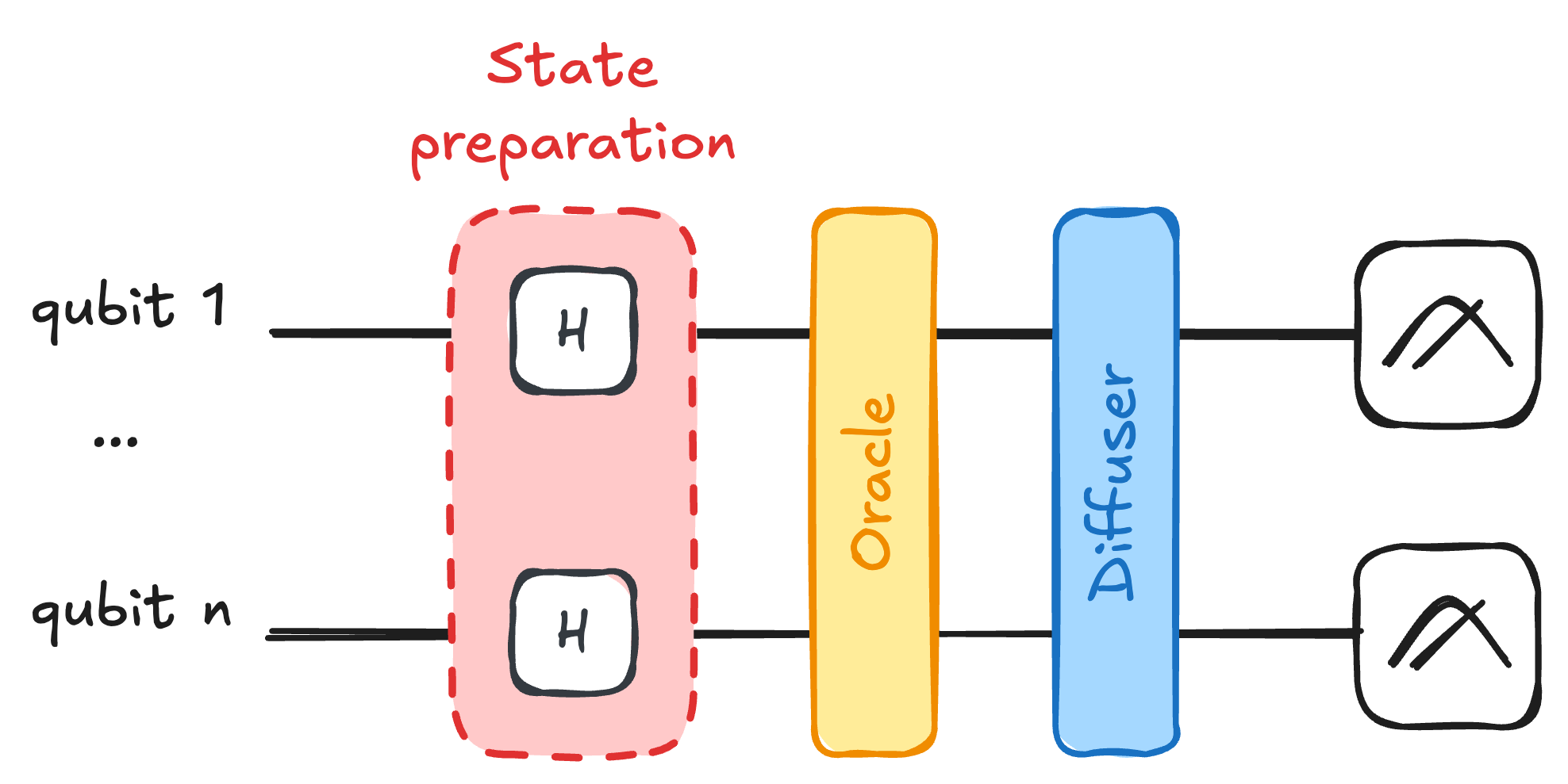
See Fig. for the circuit structure for Grover's algorithm.
The circuit begins by the state preparation phase in red with Hadamard gates creating the uniform superposition, followed by the oracle (yellow) marking the winner state, and then the diffusion operator (blue) that amplifies the marked state's amplitude.
For small databases like
For other settings, we need to repeat Oracle+Diffuser.
Let's go through all the steps of this algorithm one by one.
The Initial Superposition
Since we have no prior knowledge about which item is the winner, we begin by preparing a uniform superposition over all
This is achieved by applying Hadamard gates, introduced in the first lecture, to each of the
At this stage, if we were to measure immediately, each outcome
The probability of successfully finding the winner in a single shot is therefore
To see why this is problematic, consider that the expected number of queries
Our goal is thus to transform this uniform distribution into one heavily concentrated on
The Oracle or the Yes/No Verifier Blackbox Function
We emphasize that Grover's algorithm does not search through items one by one.
Instead, it assumes we already have access to a function that can verify whether a given input is the solution, and uses quantum interference to amplify the correct answer.
Grover's algorithm does not "look inside" the database.
Rather, it relies on an oracle, a black-box function that can recognize the winner when presented with it.
The oracle's job is simple: given any state
This distinction between finding and verifying is fundamental in complexity theory.
Recall from lecture 1 that many problems in the class NP (Non-deterministic Polynomial time) are hard to solve but easy to verify.
One example to understand this subtle difference is to consider Sudoku.
Checking whether a completed grid is valid takes seconds, but finding the solution from scratch can be much harder.
Grover's algorithm exploits this asymmetry, working for any problem where verification is efficient.
To get some intuition of what the oracle is, let's go through multiple definitions and interpretations.
Mathematical Definition of the Oracle
As we just mentioned, the oracle
This can be written compactly as
In matrix form, for a 2-qubit system where the winner is
Notice that only the diagonal entry corresponding to the winner state carries a
This phase flip is invisible if you measure immediately (the probabilities
For a 3-qubit system (
Verify that
The oracle matrix is diagonal with all entries equal to 1 except for the entry corresponding to
To verify unitarity, note that
Then:
Show that for a database of size
What is the variance of the number of queries?
Let
Then
Expected value:
Variance:
Building the Oracle from a Classical Function
Another way to get intuition on this oracle function is to express it from a classical function.
Indeed, in practice, we construct the oracle from a classical boolean function
The oracle's action can then be written as
But how do we actually implement this phase flip using quantum gates?
The standard approach uses phase kickback.
Suppose we have a quantum circuit
The trick is to prepare the target qubit not in
When we apply
If
But if
The result is:
The phase has been "kicked back" onto the input register, while the target qubit is left unchanged (up to a phase we can ignore).
This is the standard technique for converting any classical verification function into a quantum phase oracle.
Let's explain it in more details.
Phase Kickback: The Underlying Oracle Mechanism
To understand this more generally, consider a controlled-
Phase kickback occurs when a controlled operation acts on an eigenstate of the target unitary.
The eigenvalue phase gets transferred to the control qubit's relative phase.
If the control qubit starts in a superposition:
The target qubit remains in
This mechanism allows us to extract information about
Consider the controlled-
Show that the phase gets kicked back to the control qubit.
What is the resulting state?
The
Applying the controlled-
The target remains
Consider a 2-qubit system with winner
The oracle flips only the phase of
Notice that all amplitudes remain
Geometric Interpretation of Grover's Algorithm
We have not yet covered all the 3 steps of Grover's algorithm, we are still missing the Diffuser one.
But before diving into this last part, we take a moment to focus on a geometric interpretation that will help us introduce this last part.
Grover's algorithm is indeed best understood through geometry.
The key insight that we will discover is that two reflections compose to give a rotation, a fact from elementary geometry that becomes the engine of Grover's quantum speedup.
See Fig. for an step-by-step illustration of how amplitudes evolve during Grover's algorithm.
Before the oracle, all states have equal positive amplitude.
After the oracle, the winner state's amplitude becomes negative, creating an asymmetry.
The diffusion operator then reflects all amplitudes about their mean, dramatically boosting the winner's amplitude while slightly decreasing all others.
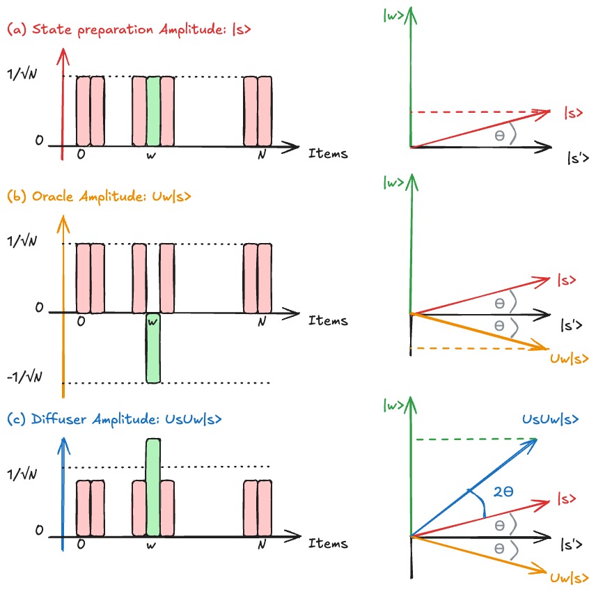
Setting Up the 2D Subspace
Let's focus on the top row of Fig..
Although our Hilbert space has dimension
: the target state we wish to find : the uniform superposition over all non-winner states, defined as
The initial state
Since
More precisely, we can write any state in this subspace as:
For the initial state, the angle from the
This tiny angle (roughly
For
The approximation gives:
The error is about 1%, which is acceptable for large
Step 1: the Oracle as a Reflection
Now let's switch to the second row of Fig..
We mentioned several interpretations for the oracle
The oracle
Geometrically, if you picture
The effect is simple: if the state was at angle
The distance to
Verify that
Using
Case 1: When
Since
Therefore:
Case 2: When
Since
This confirms that the oracle acts as a reflection about the hyperplane perpendicular to
Step 2: The Diffusion Operator as a Second Reflection
Now we briefly mention the diffuser's geometric action to understand its effect intuitively.
As can be seen in the last row of Fig., the diffuser is a second reflection, now performed about the initial state
For a 2-qubit system (
First calculate
Then:
The Diffusion Operator: Amplifying the Marked State
After applying the oracle, our quantum state looks similar to where we started, at least on the surface.
Indeed, if we measured at this point, we would still get each outcome with equal probability, since
But what is crucial is that every amplitude remains
| State | ... | ||||
|---|---|---|---|---|---|
| Amp. Before Oracle | ... | ||||
| Amp. After Oracle | ... | ||||
| Goal | 0 | 0 | ... | 1 | 0 |
The final step is the diffusion operator
As we just saw geometrically, this operator reflects all amplitudes about their average value
Mathematically, the diffusion operator is defined as:
where
The full Grover's algorithm is composed of the oracle and diffuser, but how many times?
We repeat it to get as close as possible to the winner state
The difference in signs betweenn
Mathematically, both operators perform the exact same geometric action: reflection about an axis.
The general formula for reflecting a vector across an axis defined by a projector
Here is why the signs look different for the two operators:
The Diffuser (
We have the projector for this axis:
Using the standard formula:
(This is a standard reflection about the vector
The Oracle (
Its projector is
Using the standard formula, the operator should be:
However, we don't build the circuit using "non-winners"; we build it using the winner
We know that the sum of projectors in the space must be the Identity:
Substitute this into our reflection formula:
Summary: The sign flips because of the basis we use to write the operator.
Iteration and Optimal Stopping
The following Fig. builds on Fig. and depicts the geometric view of the full Grover's algorithm in the 2D subspace spanned by
Composing these two reflections produces a rotation by
The amplitude of the winner state grows while all other amplitudes shrink, this is the amplification we sought.
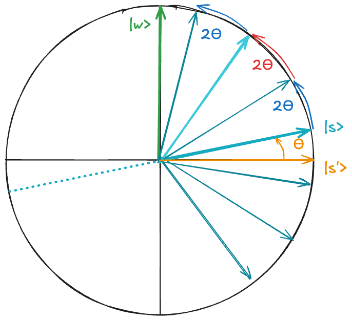
We want to stop when this angle reaches approximately
This can be see as
Solving
This is the origin of the
Each iteration rotates by a tiny angle
Calculate
Using
: vs classical (no advantage) : vs classical (2.7× speedup) : vs classical (5.3× speedup) : vs classical (9.8× speedup)
The success probability after
For
Which value of
For
: (50%) : (91%) : (99.7%) ← optimal : (73%) (over-rotated!)
The optimal is
For a database of
Compared to the classical
Unlike classical algorithms where more iterations can lead to better results, Grover's algorithm has a "sweet spot."
If you iterate beyond
You must measure at the right moment.
Generalization: Multiple Winners
We briefly mention the case where multiple states are considered as winners.
The algorithm extends naturally to the case where there are
We redefine the "winner state" as the uniform superposition over all solutions:
The geometric picture remains the same, but now the initial angle is larger:
Since we start closer to the target subspace, fewer iterations are needed:
This makes sense: if half the items are winners (
For a 4-qubit system (
Compare this to the single-winner case (
For
Optimal iterations:
For comparison, single winner (
With more winners, we start closer to the target and need fewer iterations.
Consider a 3-qubit system (
- Write down the initial state
after applying Hadamards. - Design an oracle that marks both winning states (hint: it should flip the phase of
and ). - Calculate the initial angle
and determine the optimal number of iterations. - Draw the quantum circuit.
1. Initial state:
After applying Hadamard gates to all three qubits starting from
2. Oracle design:
The oracle must flip the phase of both
In matrix form, this is a diagonal matrix with entries:
The oracle can be implemented as a combination of controlled gates that detect both patterns.
3. Initial angle and optimal iterations:
With
Optimal number of iterations:
Only one iteration is needed!
4. Quantum circuit:
The circuit consists of:
- Initialization: Three Hadamard gates on qubits 0, 1, 2
- Oracle: A multi-controlled gate structure that flips the phase when the state is either
or - Diffuser:
, followed by a multi-controlled Z gate (with X gates on controls to detect ), then again - Measurement: Measure all three qubits
The oracle can be decomposed as:
Oracle = (CZ on qubits that detect |101⟩) + (CZ on qubits that detect |110⟩)
Understanding the Amplitude Dynamics: Inversion About the Mean
The geometric picture is clear, but it's also helpful to see how the amplitudes evolve algebraically.
This reveals the mechanism of "inversion about the mean" that gives the diffusion operator its amplifying power.
The final state after one iteration is:
After applying the oracle, the state becomes
Let's compute what happens when we apply the diffusion operator
Using the fact that
The key observation is that
After some algebra, the amplitude of state
| State | New Amplitude | Effect | ||
|---|---|---|---|---|
| Loser | 0 | +1 | From |
|
| Winner | 1 | -1 | From |
The winner's amplitude roughly triples with each iteration (for large
This is the quantitative manifestation of "inversion about the mean": the winner amplitude, being far below the mean, gets reflected far above it.
The Physical Origin of Interference
To finish discussing the algorithm and before switching to examples and experimental realisations, let's wonder where the quantum interference takes place.
You remember from previous lecture that a quantum computer's advantage does not rely in running the same calculation in parallel over all the superposed states.
Rather, you only want a single state in your final state distribution.
The speedup in Grover's algorithm comes from this quantum interference, and it's worth understanding where this interference arises:
- The Oracle Step:
- By flipping the winner's phase to negative, the oracle creates a situation where the winner amplitude is now "out of step" with all the others.
- The mean amplitude drops slightly because of this negative contribution.
- The Diffusion Step: The diffusion operator reflects all amplitudes about this new (lower) mean.
- For the loser states, which sit just above the mean, reflection barely moves them.
- But the winner state sits far below the mean, so reflection pushes it upward, effectively collecting constructive contributions from all the other states, the
factor we saw in the previous section.
This is constructive interference for the winner and destructive interference for the losers, achieved not by path differences (as in optical interference) but by manipulation of quantum phases.
Where does the speedup come from? You can see it from Pythagoras' theorem.
In the classical world, different observable states are like pure coordinate directions (the axes of our Hilbert space). To get from your starting point to the correct answer, you are essentially "walking the edges" of an
- Classical (Manhattan distance): You have to traverse
items one by one. You are constrained to move along the axes (checking one bit string at a time). To reach the "opposite corner" of a unit cube in dimensions, you would have to walk units. Distance . - Quantum (Euclidean distance): Quantum mechanics gives us access to diagonal directions (superpositions) that are unavailable to a classical system.
- By allowing the state vector to move "diagonally" through the Hilbert space, we can take a shortcut.
- In an
-dimensional space, the distance from the origin to the opposite corner is . - The Grover iteration effectively traces a quarter-circle arc from our initial state to the target, utilizing these "diagonal" states to achieve a square-root shortcut.
- The state vector slowly walks along this arc, taking a path that would be entirely unavailable if we were limited to pure coordinate directions.
It is proven (see BBBV Theorem) that
When we will discuss resource estimation and space-time overhead (how many qubits and how much time) of applications, we will see that the
The "Quadratic Trap" occurs when the quantum computer's clock speed is slower than the classical computer.
If the "Quantum constant"
Said in another way:
If
Example: 2-Qubit Search (
Let's work through Grover's algorithm for the smallest non-trivial case: searching among 4 items with 2 qubits.
In this example, we'll suppose the winner is
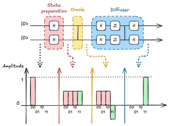
Initial Setup
The starting angle is
Since we need to rotate from
This is a special case where a single Grover iteration gives perfect success probability.
The Oracle
For winner state
In matrix form, this oracle is simply the controlled-Z gate:
Implementing the Diffusion Operator
The diffusion operator
The key insight is that reflecting about
- Rotating
to : - Reflecting about
: - Rotating back:
Where
The operator
For 2 qubits, this decomposes to
The complete circuit has three stages: Initialization (Hadamards to create
A more complex example with 5 qubits and one winner can be seen using Quirk.
Qiskit Examples
Let's look at examples that you can run yourself.
Examples with 2 And 3 Qubits
First go to Colab, a colaborative jupyter notebook website.
Then click on "Open Notebook" for a new Colab notebook and paste the Github url from a Grover implementation edited from the official qiskit release: qiskit-demo/presentations/grover.ipynb at main · francois-marie/qiskit-demo.
Application: Sudoku
How would you encode a
Let's do this using Qiksit and Colab!
Experimental Implementations
We end this first part of the lecture by looking at some experimental implementations.
Grover's algorithm has been demonstrated on many quantum computing platforms: historically NMR but also superconducting (SC), trapped ions, photonics, and spins.
The table below summarizes key experimental results, showing the gap between theoretical and achieved success probabilities, a measure of hardware quality.
| Platform | Reference | Qubits | Database items | Winners | Exp. Success Rate | Theo. Success Rate |
|---|---|---|---|---|---|---|
| SC | 4 | 3 | 8 | - | - | |
| SC | 5 | 6 | 64 | - | 4% | |
| SC | 5 | 4 | 32 | - | 45% | |
| Trapped Ions | 6 | 3 | 8 | 1 | 0.39 | 0.78 |
| Trapped Ions | 6 | 3 | 8 | 2 | 0.70 | 1 |
| Photonics | 7 | 2 | 4 | 1 | 0.71 | |
| Silicon Spins | 8 | 3 | 8 | 1 | 0.93 | 0.98 |
| Silicon Spins | 8 | 3 | 8 | 2 | 0.96 | 1 |
| NMR | 2 | 2 | 4 | 1 | - |
Notice that silicon spin qubits achieve high fidelities, approaching theoretical limits.
The gap between achieved and theoretical success rates reflects gate errors and decoherence in current hardware.
Quantum Fourier Transform and Phase Estimation
Having explored Grover's quadratic speedup for unstructured search, we now turn back to last week's lecture, to a different class of algorithms that achieve exponential advantages.
The Quantum Fourier Transform and Quantum Phase Estimation are the workhorses behind Shor's factoring algorithm but also quantum chemistry simulations, and many other applications.
While Grover taught us about amplitude amplification through geometric rotations, QFT and QPE reveal how quantum computers can extract hidden periodicities and eigenvalues exponentially faster than classical approaches.
Classical Fourier Transform
Let's start by recalling some intuition on the Fourier transform.
The Fourier transform is one of the most powerful tools in mathematics and engineering.
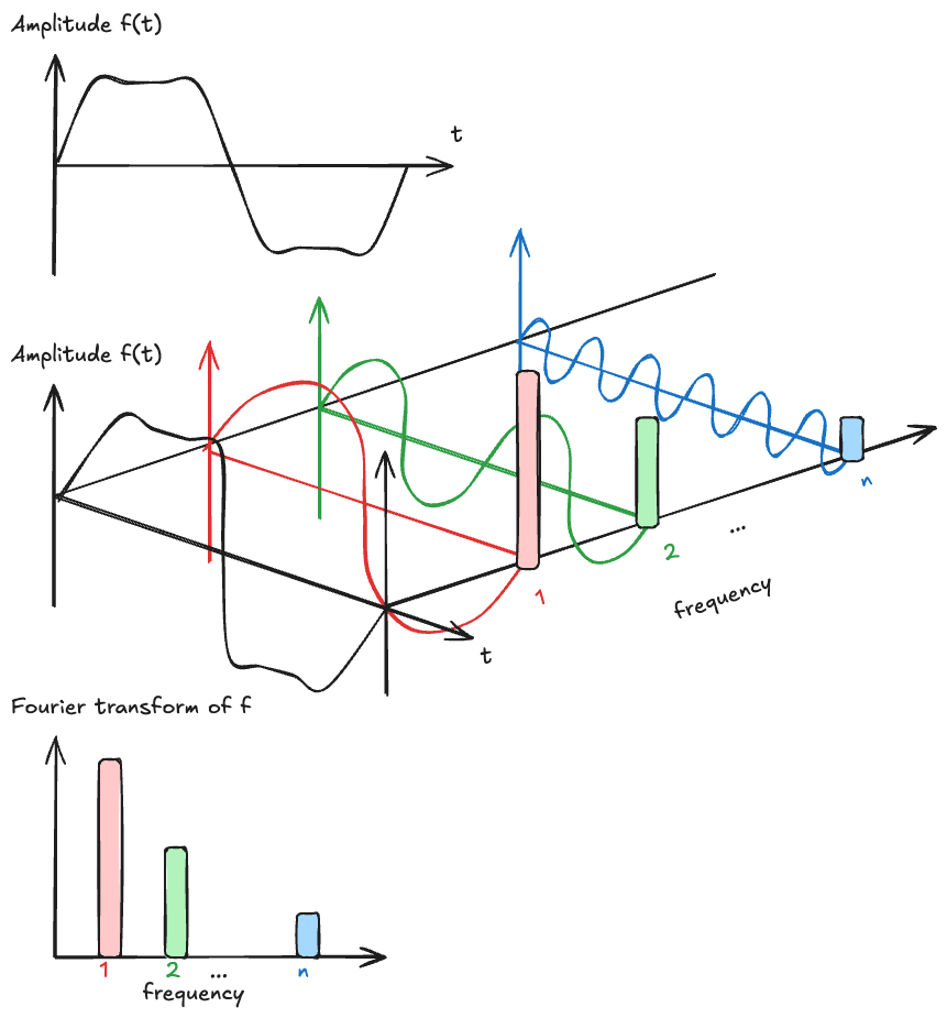
It converts signals from the time domain to the frequency domain, revealing hidden periodicities, see Fig. that illustrates the concept of Fourier transformation, adapted from Wikipédia's page on the Fourier transform.
A time-domain signal
The Fourier transform reveals the amplitude and phase of each frequency component (bottom row), making hidden periodicities visible.
The key insight is that periodic structure in the time domain becomes localized peaks in the frequency domain.
Mathematically, the transform
The quantum version performs this transformation on quantum amplitudes rather than classical signals but the idea remains the same.
The classical Fast Fourier Transform (FFT) on
The Quantum Fourier Transform on
Compare these complexities for
For
- Classical FFT:
operations - QFT:
gates
Comparison:
| Classical: |
Quantum: |
Speedup Factor | ||
|---|---|---|---|---|
| 10 | 1,024 | 10,240 | 100 | 100× |
| 20 | 1,048,576 | 20,971,520 | 400 | 52,000× |
| 30 | 900 |
Discrete Fourier Transform (DFT)
For computational purposes, we can work with discrete vectors rather than continuous functions.
Given an input vector
The quantity
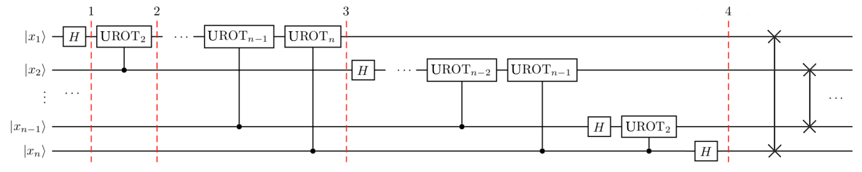
The Quantum Fourier Transform
Going from DFT to QFT is simply switching from vectors to vector states: the QFT performs the DFT on the amplitudes of a quantum state.
If we start with a state
For a computational basis state
The QFT creates a superposition where each basis state
Matrix Representation
Mathematically, the QFT can be expressed as an
Each row represents a different "frequency", and the entries oscillate faster as you move down the matrix.
For
Verify that the first column corresponds to
Using
The first column is
Key Properties
For the sake of completeness, we briefly mention some key properties of the QFT.
The QFT is a unitary transformation:
This means it preserves probability (as all quantum operations must) and is reversible.
The inverse QFT is simply
Let
Calculate
Show that
For the sum with
This orthogonality property is crucial for the QFT.
Building Intuition: How the QFT Encodes Information
Before diving into the circuit representation of the QFT, we build some intuition by looking at an example of QFT on basis states.
A feature of the QFT is that when applied to a basis state
As we will see explicitly by taking the example of 3 and 4 qubits, each output qubit is in a superposition
In binary notation, where
The different qubits rotate at different "frequencies":
- The least significant output qubit rotates by
between consecutive inputs (fastest oscillation) hence oscillates between and , - The next qubit rotates by
(half the frequency), hence oscillates between - Each subsequent qubit rotates half as fast
This hierarchical structure of phases is what makes the QFT useful for detecting periodicity (on what relies Shor's algorithm): if the input state has period
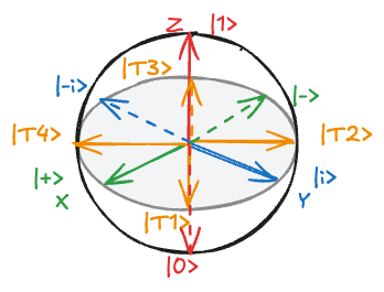
As shown in Fig., the QFT output states can be visualized on the Bloch sphere with their phase relationships. Let's map explicitly input number states to their binary representations and QFT outputs in the following table:
| Input state | Binary |
QFT Output |
|---|---|---|
The first qubit oscillates from
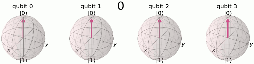
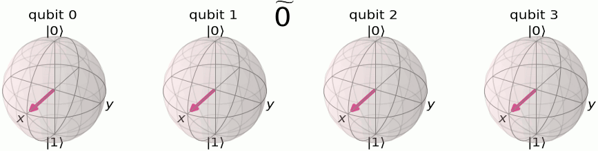
In Fig. and Fig., we can see this even more clearly on 4 qubits, where the first qubit oscillates between
The pattern reveals how the input number
For the 3-qubit state
- The fastest qubit (
) rotates by - The middle qubit (
) rotates twice as slowly: - The slowest qubit (
) rotates at half that rate:
Let's write the full explicit tensor product form for QFT on
Calculate the explicit product state representation for
Express your answer as a tensor product of single-qubit states
For
The phases for each output qubit are:
- Qubit 1 (slowest):
- Qubit 2 (middle):
- Qubit 3 (fastest):
Therefore:
Now that we built some intuition on what the QFT does in practice, let's look at its circuit implementation.
QFT Circuit Implementation
The feature of the QFT is that it can be implemented with only
The circuit uses two types of gates:
Hadamard gate: Creates equal superposition of
Controlled phase rotation: Adds a phase depending on the control qubit:
The circuit of Fig. illustrates the complete circuit structure and applies Hadamards and controlled rotations in a specific pattern, followed by SWAP gates to reverse the qubit order.
The algorithm proceeds as follows:
- apply a Hadamard to the first qubit, then controlled-
(controlled by qubit 2), controlled- (controlled by qubit 3), and so on. - Then move to the second qubit and repeat with smaller rotations.
For an
How many Hadamard gates, controlled rotation gates, and SWAP gates are needed?
What is the total circuit depth (assuming all gates are sequential)?
For each of the
- Qubit 1: 1 Hadamard +
controlled rotations - Qubit 2: 1 Hadamard +
controlled rotations - Qubit
: 1 Hadamard + controlled rotations
Total gates:
- Hadamards:
- Controlled rotations:
- SWAPs:
(to reverse qubit order)
Circuit depth:
With approximations, this can be reduced to
A nice and interactive display of the QFT circuit on 8 qubits can be found on Quirk.
The Inverse QFT
Since the QFT is unitary, we briefly mention that its inverse
In terms of circuit implementation, the inverse QFT circuit is simply the original circuit run backwards: reverse the order of all gates and replace each
The inverse QFT is important for extracting classical information from quantum phase information, we now focus on this in action in Quantum Phase Estimation use case.
Describe the circuit for the inverse QFT on 3 qubits.
What are the gate types, and in what order do they appear?
How does it differ from the forward QFT circuit?
The inverse QFT circuit reverses the forward QFT:
Forward QFT (3 qubits):
- SWAPs (if bit-reversal needed)
on qubit 3, then controlled by qubits 2,1 on qubit 2, then controlled by qubit 1 on qubit 1
Inverse QFT (3 qubits):
on qubit 1 controlled by qubit 1 on target qubit 2, then on qubit 2 controlled by qubit 1, then controlled by qubit 2, then on qubit 3 - SWAPs (reversed)
The inverse uses
Do it Yourself!
Just like for Grover's algorithm, let's look at examples that you can run yourself.
Go again to Colab, a colaborative jupyter notebook website.
Then click on "Open Notebook" for a new Colab notebook and paste the following Github url: qiskit-demo/presentations/quantum-fourier-transform.ipynb at main · francois-marie/qiskit-demo.
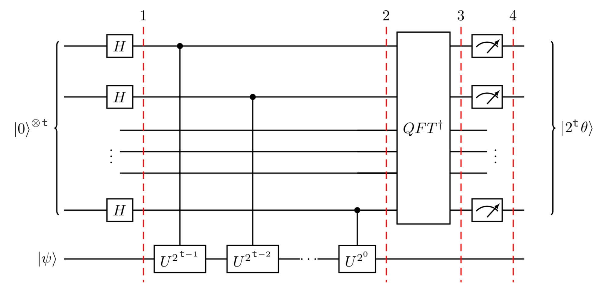
Application: Quantum Phase Estimation (QPE)
The QFT finds one of its most important application in Quantum Phase Estimation, a subroutine used by Shor's factoring algorithm and many quantum chemistry algorithms.
Let's start by quickly explaining the problem at stake.
The Problem
You are given a unitary operator
Looks pretty straightforward, right?
But how would you do this in practice?
The Key Insight: the return of the Phase Kickback
QPE uses controlled-
If we apply
We see that by using multiple control qubits with different powers of
The circuit implementation is shown in Fig.:
Suppose
Calculate the phase acquired by the control qubit when applying
Express your answer as
Since
Applying the controlled operation:
The phase is:
Therefore the control qubit acquires phase
The depicted circuit above can be hard to understand so to make things hopefully clearer, let's take an example.
Consider the
The state
Thus
If we run QPE with 3 qubits in the auxiliary register, the algorithm will encode
After the inverse QFT, we measure the auxiliary register and obtain the binary representation of
This example illustrates the power of QPE: it converts quantum phase information, which is normally invisible to measurement, into a classical bitstring that we can read out directly.
What would you measure if you used only 2 qubits in the auxiliary register instead of 3?
Would the result still be exact?
We can only represent
The exact value
Measurement would give
We need at least
In QPE, the auxiliary register has
If we want to estimate a phase
What is the probability of success if we use exactly this many qubits?
To achieve accuracy
Since each qubit adds one bit of precision (halving the uncertainty), we need:
Example: For
Success probability: If
If not, the standard QPE algorithm has success probability
To achieve high success probability (
Qiskit time
We end this section by running some code.
Just like for Grover's algorithm and QFT, let's look at examples that you can run yourself.
Go again to Colab, a colaborative jupyter notebook website.
Then click on "Open Notebook" for a new Colab notebook and paste the following Github url: qiskit-demo/presentations/quantum-phase-estimation.ipynb at main · francois-marie/qiskit-demo.
Resource Estimates
Between last week's lecture and today's, we've now seen two paradigms of quantum advantage: Grover's quadratic speedup for search and the exponential speedup of Shor, QFT and phase estimation.
But there's a crucial question we haven't addressed yet.
Can we actually run these algorithms on real hardware?
How many would would we need and how much time would it take to run a useful quantum application?
Answering these questions provides what's called space-time overheads and is crucial to understand the cost of quantum advantage.
The answer depends not just on the number of logical (aka perfect and noiseless) qubits required, but on error rates and coherence times of physical qubits, and the massive overhead of quantum error correction that we will discuss in the next two lectures.
Let's end this lecture by confronting the resource requirements and understand the gap between algorithmic promise and experimental reality.
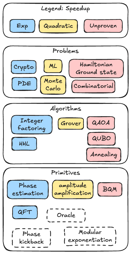
(Partial) Landscape of Quantum Algorithms
We've said already that different problem classes admit different types of quantum speedups, see Fig.:
- Problems like factoring, discrete logarithm, or HHL algorithm where quantum computers achieve exponential advantage (in blue),
- Optimization and search problems where we see quadratic speedups (yellow),
- Other types of problems, like finding the ground state of an Hamiltonian or combinatorial problems, with an unproven advantage (red)
To classify all these quantum applications, we first decompose them in terms of the algorithm they use (for instance, remember that Grover's algorithm is at the center of a wide variety of use cases) and the primitives or building blocks of the algorithm.
More detailed maps exist but they become quickly unreadable.
However, considering even such a partial landscape allows to take a step back on the many topics addressed during our two "Application" lectures and all of the many remaining ones that you will discover in your future careers.
Resource Overheads: From Theory to Reality
Let's talk numbers.
When researchers publish quantum algorithms, they often focus on asymptotic complexity (the
But if you want to actually run these algorithms on hardware one day, you need concrete resource estimates beforehand.
How many qubits? How many gates? How long will it take? What error rates can we tolerate?
Take nitrogen fixation as an example.
For context, the FeMoCo (iron-molybdenum cofactor) is the active site in certain bacteria that can convert atmospheric nitrogen into ammonia at room temperature.
If we could understand this process well enough to replicate it industrially, we could revolutionize agriculture and reduce the massive energy costs of the Haber-Bosch process.
Quantum simulation of FeMoCo is often cited as a "killer app" for quantum computers because the electronic structure involves strongly correlated electrons that are extremely difficult for classical computers to handle accurately.
But here's the reality check.
Even for this relatively small molecule (Fe
Besides, that's not 100-1000 physical qubits (that we can build that today), but error-corrected logical qubits, each potentially requiring thousands of physical qubits depending on your error correction code and the quality of your hardware (more on that next week).
The tradeoff between circuit depth (number of sequential gates) and width (number of qubits) depends on the specific problem and algorithm.
Financial optimization problems can require even more qubits (around 10,000 logical qubits) but fewer total gates.
For Shor's algorithm attacking RSA-2048 (the encryption standard used widely on the internet), you need about 1,000 logical qubits.
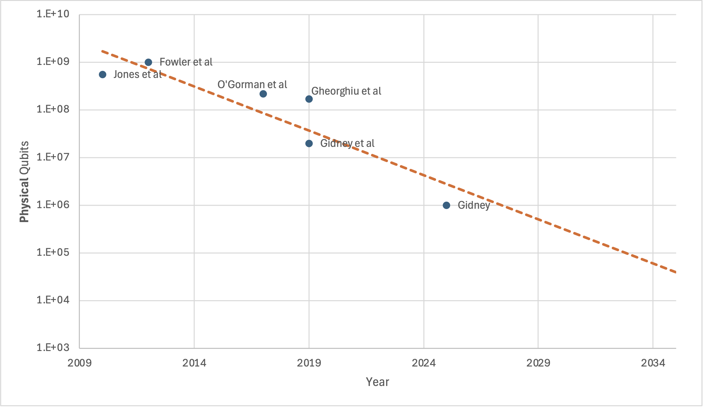
But when you account for quantum error correction, that balloons to roughly 1 million physical qubits for the Gidney estimate 9, or 20 million for more conservative assumptions or other platforms 10.
And you would need to run the computation for about a week, maintaining coherence and performing error correction continuously throughout.
| App. | FeMoCo (Chemistry) 11 | Financial opti. 12 | RSA-2048 (Shor, SC) 9 | RSA-2048 (Shor, NA) 10 |
|---|---|---|---|---|
| Logical Qubits | ||||
| Logical Gates | ||||
| Physical Qubits | - | - | ||
| Runtime | Days to months | ~1 week | ~1 week |
Bridging Theory and Practice
The gap between what we can build and what we need is real, but it's closing.
See Fig. from Quantum Landscape which shows historical progress in reducing resource estimates for problems related to cryptography.
Back in the early 2000s, estimates for factoring RSA-2048 were in the billions of qubits.
Today, through better algorithms and more efficient error correction schemes, we're down to the millions.
That's still far from the hundreds or thousands of qubits in current machines, but the trajectory is clear.
Will this be sustainable or will it plateau? Still an open question.
Where We Stand Today
Also from Quantum Landscape, Fig. provides a snapshot of where we are right now.
Current quantum processors have somewhere between 100 and 1,000 physical qubits, depending on the platform.
Superconducting qubits (IBM, Google, Rigetti) are pushing toward the high hundreds.
Trapped ions (IonQ, Quantinuum) have fewer qubits but better connectivity and gate fidelities.
Neutral atoms (QuEra, Pasqal) can scale to larger numbers but are still working on gate fidelities.
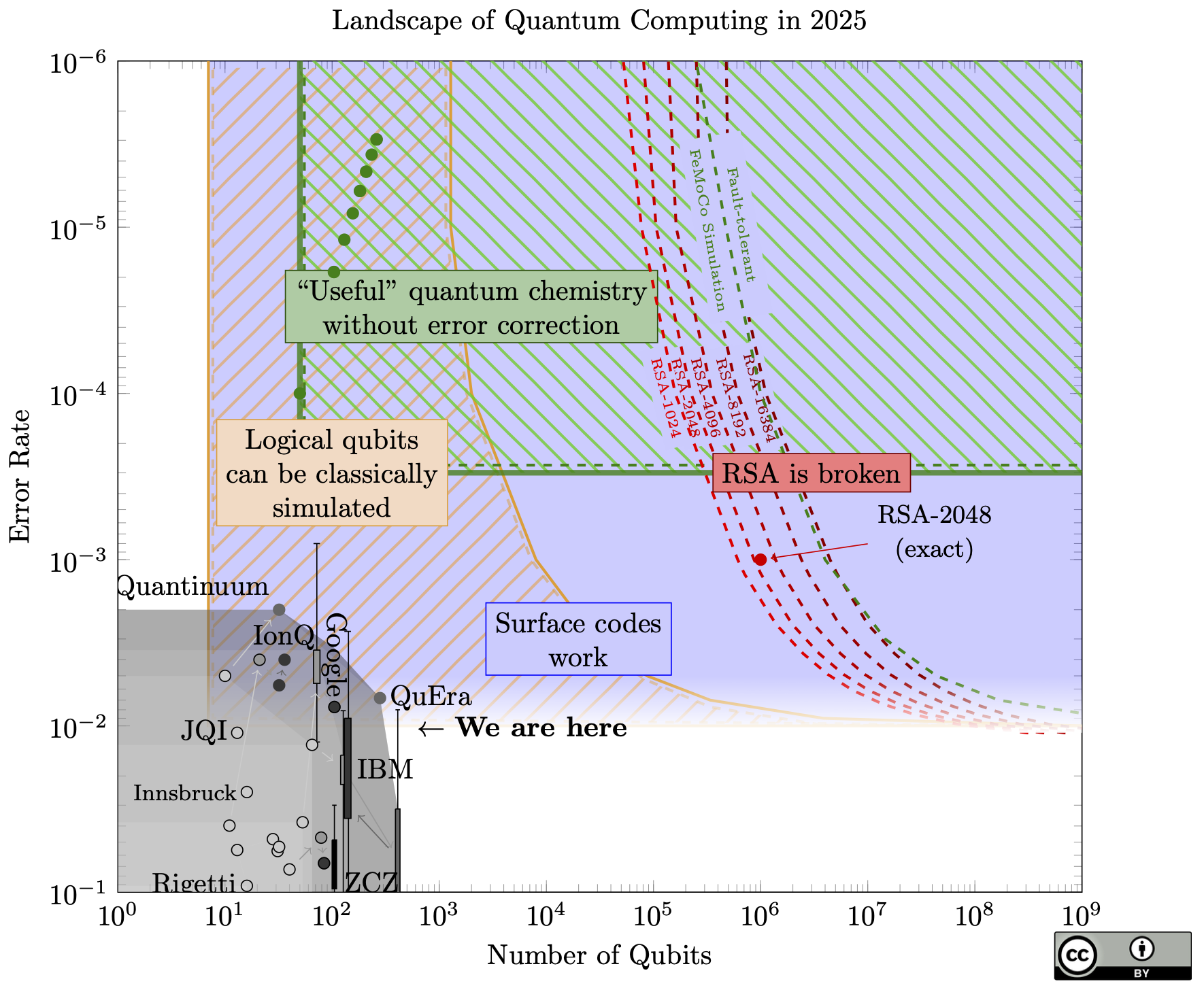
The vertical axis in this figure is linked to the number of logical operations you can perform reliably.
Right now, we're in the NISQ (Noisy Intermediate-Scale Quantum) era, meaning we have devices with somehow a decent number of qubits but not enough coherence or low enough error rates to implement reach what is needed for useful algorithm, on the order of
We can run short circuits (maybe a few hundred to a thousand gates) before errors accumulate and destroy the computation.
But look at where the useful algorithms sit.
Shor's algorithm needs millions of gates.
Quantum chemistry simulations need even more.
The applications that would provide clear practical advantage are still out of reach compared to today's achieved performance.
Even if we can increase the number of qubits, useful computations would still be out of reach because of the error rates gap between what we have and what is required.
This is precisely why quantum error correction is the next major topic in this course: building one almost-noise-free qubit out of many noisy ones.
QEC is the bridge the gap between NISQ devices and fault-tolerant quantum computers that can run Shor, simulate molecules, and tackle the problems we've been discussing.
Without error correction, we're limited to small demonstrations and variational algorithms that try to squeeze utility out of noisy circuits.
With error correction, we unlock the full algorithmic power of quantum computing.
The Path Forward
The takeaway of this section isn't pessimism, it's realism.
Quantum algorithms provide genuine speedups (quadratic for Grover, exponential for Shor and quantum simulation).
But translating those asymptotic advantages into practical utility requires overcoming significant engineering challenges.
We need:
- Better qubits: Lower error rates, longer coherence times
- More qubits: Scaling from hundreds to millions
- Error correction: Efficient codes that don't require prohibitive overhead
- Compilation and optimization: Smarter ways to map algorithms onto hardware constraints
The next lectures on quantum error correction will show you exactly how we plan to get there.
We'll see how the surface code and other QEC schemes can protect quantum information from noise, how to perform fault-tolerant gates on encoded qubits (aka robust to physical error propagating), and what it will take to reach the thresholds where error-corrected quantum computing becomes viable.
The resource estimates we've discussed today aren't fixed targets but they're moving goals that improve and get closer to reality as we develop better codes, better compilers, and better hardware.
But they give you a realistic picture of where the field stands and what needs to happen next.
Conclusion
In this lecture, we've explored three pillars of the quantum algorithm landscape.
Grover's algorithm showed us how quantum interference and geometric rotations in Hilbert space can achieve a quadratic speedup for unstructured search, with the insight that two reflections compose into a rotation.
The Quantum Fourier Transform revealed how quantum computers can extract periodicities exponentially faster than classical FFTs, by encoding information into relative phases of product states.
And Quantum Phase Estimation demonstrated how phase kickback and the inverse QFT can convert hidden eigenvalue information into measurable classical bits, powering applications from factoring to quantum chemistry.
But we also confronted a sobering reality.
The gap between theoretical speedups and practical implementations remains vast.
Shor's algorithm can break RSA-2048 in polynomial time, but doing so requires millions of physical qubits and weeks of coherent operation.
This gap isn't a fundamental limitation, it's an engineering challenge.
In the upcoming lectures, we'll see how quantum error correction works to bridge this gap, starting with simple repetition codes and building up to the surface code and other codes that are the leading candidates for fault-tolerant quantum computing.
We'll understand the threshold theorem that proves error correction can work even with imperfect gates, and we'll see what it takes to perform logical operations on encoded qubits without destroying the error protection.
References
- 1.
- Chen, Z; Satzinger, K; Atalaya, J; Korotkov, A; Dunsworth, A; Sank, D; Quintana, C; McEwen, M; Barends, R; Klimov, P; Hong, S; Jones, C; Petukhov, A; Kafri, D; Demura, S; Burkett, B; Gidney, C; Fowler, A; Paler, A; Putterman, H; Aleiner, I; Arute, F; Arya, K; Babbush, R; Bardin, J; Bengtsson, A; Bourassa, A; Broughton, M; Buckley, B; Buell, D; Bushnell, N; Chiaro, B; Collins, R; Courtney, W; Derk, A; Eppens, D; Erickson, C; Farhi, E; Foxen, B; Giustina, M; Greene, A; Gross, J; Harrigan, M; Harrington, S; Hilton, J; Ho, A; Huang, T; Huggins, W; Ioffe, L; Isakov, S; Jeffrey, E; Jiang, Z; Kechedzhi, K; Kim, S; Kitaev, A; Kostritsa, F; Landhuis, D; Laptev, P; Lucero, E; Martin, O; McClean, J; McCourt, T; Mi, X; Miao, K; Mohseni, M; Montazeri, S; Mruczkiewicz, W; Mutus, J; Naaman, O; Neeley, M; Neill, C; Newman, M; Niu, M; O’Brien, T; Opremcak, A; Ostby, E; Pató, B; Redd, N; Roushan, P; Rubin, N; Shvarts, V; Strain, D; Szalay, M; Trevithick, M; Villalonga, B; White, T; Yao, Z; Yeh, P; Yoo, J; Zalcman, A; Neven, H; Boixo, S; Smelyanskiy, V; Chen, Y; Megrant, A; Kelly, J . Exponential suppression of bit or phase errors with cyclic error correction. Nature 595 (7867) , 383–387 (2021) . doi:10.1038/s41586-021-03588-y
- 2.
- Chuang, I; Gershenfeld, N; Kubinec, M . Experimental Implementation of Fast Quantum Searching. Physical Review Letters 80 (15) , 3408–3411 (1998) . doi:10.1103/PhysRevLett.80.3408
- 3.
- Grover, L . A fast quantum mechanical algorithm for database search. Proceedings of the twenty-eighth annual ACM symposium on Theory of Computing , 212–219 (1996) . doi:10.1145/237814.237866
- 4.
- AbuGhanem, M . Characterizing Grover search algorithm on large-scale superconducting quantum computers. Scientific Reports 15 (1) , 1281 (2025) . doi:10.1038/s41598-024-80188-6
- 5.
- Chu, J; He, X; Zhou, Y; Yuan, J; Zhang, L; Guo, Q; Hai, Y; Han, Z; Hu, C; Huang, W; Jia, H; Jiao, D; Li, S; Liu, Y; Ni, Z; Nie, L; Pan, X; Qiu, J; Wei, W; Nuerbolati, W; Yang, Z; Zhang, J; Zhang, Z; Zou, W; Chen, Y; Deng, X; Deng, X; Hu, L; Li, J; Liu, S; Lu, Y; Niu, J; Tan, D; Xu, Y; Yan, T; Zhong, Y; Yan, F; Sun, X; Yu, D . Scalable algorithm simplification using quantum AND logic. Nature Physics 19 (1) , 126–131 (2023) . doi:10.1038/s41567-022-01813-7
- 6.
- Figgatt, C; Maslov, D; Landsman, K; Linke, N; Debnath, S; Monroe, C . Complete 3-Qubit Grover search on a programmable quantum computer. Nature Communications 8 (1) , 1918 (2017) . doi:10.1038/s41467-017-01904-7
- 7.
- Main, D; Drmota, P; Nadlinger, D; Ainley, E; Agrawal, A; Nichol, B; Srinivas, R; Araneda, G; Lucas, D . Distributed quantum computing across an optical network link. Nature 638 (8050) , 383–388 (2025) . doi:10.1038/s41586-024-08404-x
- 8.
- Thorvaldson, I; Poulos, D; Moehle, C; Misha, S; Edlbauer, H; Reiner, J; Geng, H; Voisin, B; Jones, M; Donnelly, M; Peña, L; Hill, C; Myers, C; Keizer, J; Chung, Y; Gorman, S; Kranz, L; Simmons, M . Grover’s algorithm in a four-qubit silicon processor above the fault-tolerant threshold. Nature Nanotechnology 20 (4) , 472–477 (2025) . doi:10.1038/s41565-024-01853-5
- 9.
- Gidney, C . How to factor 2048 bit RSA integers with less than a million noisy qubits. (2025) . doi:10.48550/arXiv.2505.15917
- 10.
- Zhou, H; Duckering, C; Zhao, C; Bluvstein, D; Cain, M; Kubica, A; Wang, S; Lukin, M . Resource Analysis of Low-Overhead Transversal Architectures for Reconfigurable Atom Arrays. (2025) . doi:10.48550/arXiv.2505.15907
- 11.
- Reiher, M; Wiebe, N; Svore, K; Wecker, D; Troyer, M . Elucidating Reaction Mechanisms on Quantum Computers. Proceedings of the National Academy of Sciences 114 (29) , 7555–7560 (2017) . doi:10.1073/pnas.1619152114
- 12.
- Chakrabarti, S; Krishnakumar, R; Mazzola, G; Stamatopoulos, N; Woerner, S; Zeng, W . A Threshold for Quantum Advantage in Derivative Pricing. (2021) . doi:10.48550/arXiv.2012.03819