Superconducting Circuits for Quantum Information Processing
Lecture: Engineering Superconducting Circuits
Objectives & Overview
These lecture notes provide an overview of superconducting circuits for quantum information processing, ranging from fundamental principles to advanced bosonic encoding schemes.
Our goal is to understand how we can engineer artificial atoms using macroscopic electrical circuits. We will start by establishing a physical intuition linking mechanical systems to electrical ones, then move to the non-linear elements that allow us to define qubits in superconducting circuits, and finally explore how to protect quantum information using the infinite Hilbert space of harmonic oscillators.
Here are the key themes that we will cover in this lecture:
- Quantum Harmonic Oscillator (QHO):
- Establishing the correspondence between mechanical pendulums and LC circuits
- Lagrangian and Hamiltonian formulation of circuit dynamics
- Canonical quantization and phase space representations
- The Transmon Qubit:
- Introducing the Josephson[1] Junction as a non-linear inductor to create anharmonicity.
- Deriving the Transmon Hamiltonian and the Duffing oscillator model.
- Control & Readout: Microwave drive, Rotating Wave Approximation (RWA), and dispersive readout.
- Coupling: Capacitive coupling between qubits for 2-qubit gates.
- Bosonic Encoding & Error Correction:
- Utilizing the infinite Hilbert space of harmonic oscillators for redundant encoding.
- Open Quantum Systems: Modeling dissipation with the Lindblad master equation.
- Cat Codes: Stabilizing coherent states (
) to suppress bit-flip noise. - Bias-Preserving Gates: Implementing operations that respect the noise bias structure.
- GKP Codes: Translationally symmetric codes and symplectic geometry in phase space.
These notes were written for the Experimental Quantum Computing and Error Correction course of M2 Master QLMN, see the course's website for more information.
They rely on the standard formalism of superconducting circuits typically found in 1 and for bosonic codes in 2.
Also, a really nice description of superconducting transmon qubits is accessible on the qiskit youtube channel, presented by Zlatko Minev.
3, 4, 5, 7, 9, 11, 13, 16, 17, 18
Quantum Harmonic Oscillator
Classical Harmonic Oscillator
To understand superconducting qubits, it is helpful to start with a system you already know well: the mechanical harmonic oscillator.
Recall from your earlier lectures that a simple pendulum or a mass on a spring is the foundational model for quantization.
The Hamiltonian of a 1D particle is given by
In the quantum regime, we introduced Ladder Operators:
- Annihilation operator (
): . - Creation operator (
): . - Position and Momentum relations:
and .
Action on Fock States
. . - Commutator:
.
These operators allow us to write the Hamiltonian in its quantized form,
Substitute
Show that
Now, let's translate this mechanical intuition into electrical circuit variables.
In an classical LC circuit, we don't have a mass or a spring, but we have charge and flux which behave as conjugate variables.
Electrical Variables and Physical Intuition
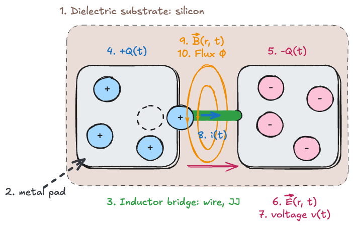
In electrical circuits, see Fig., the charge (
For a capacitor, the relationship is given by
Flux (
In the case of an inductor, the flux is
The total energy (
Specifically, the energy stored in the capacitor is
We can map the LC circuit to a pendulum in two ways:
-
Charge as Position (The "Classical" View):
- Charge
Position - Inductor
Mass (Inertia against current change ) - Capacitor
Spring constant (Restoring force from accumulated charge) - This is intuitive for classical circuits but problematic for quantum circuits with Josephson Junctions.
- Charge
-
Flux as Position (The "Quantum" View - Used Here):
- Flux
Position - Capacitor
Mass (Kinetic energy term ) - Inductor
Spring constant (Potential energy term )
- Flux
Why do we use the second one?
The Josephson Junction acts like a non-linear inductor. Its energy
Kirchhoff's Network Laws
Using the nodes and loops of the circuit we can derive the equation of motion.
Kirchhoff's Current Law (KCL) states that
Similarly, Faraday's Law of Induction (or Kirchhoff's Voltage Law) requires
Given
Derive the equation of motion
The solution describes a harmonic oscillation:
In this flux-based representation, it is the magnetic flux
The Hamiltonian for the Harmonic Oscillator
Rather than deriving the system from the Lagrangian and performing a Legendre transformation, we can obtain the Hamiltonian more directly by summing the energies stored in the elements of the circuit.
The Hamiltonian
The total energy is given by the sum of the electrostatic energy in the capacitor and the magnetic energy in the inductor:
In this expression, the term
Meanwhile,
Why are flux (
In quantum mechanics, you cannot know position and momentum simultaneously with infinite precision. Similarly, in a quantum circuit, you cannot know the exact number of Cooper pairs on the capacitor island (
To verify that
This approach allows us to recover the fundamental relations for voltage and current in the circuit.
First, consider the equation for velocity.
The time evolution of the "position" coordinate,
Taking the derivative of the Hamiltonian with respect to
Since
This equation matches the definition of magnetic flux, as voltage is the time derivative of flux according to Faraday's law.
Next, consider the equation associated with force.
The time evolution of the "momentum" coordinate
When we differentiate the Hamiltonian with respect to
Recall that the flux in an inductor is given by
Because
This result directly reflects Kirchhoff's current law for a closed LC circuit.
Combine the two results derived above (
Starting from the Lagrangian
Another way to represent this is that the electric charges on the capacitor are flowing through the inductor to the other plate and back and forth:
Using phase space representation, we can express the circular motion using
The Hamiltonian can be rewritten using
Canonical Quantization
Transitioning from classical to quantum mechanics involves promoting our variables to operators, a process known as Dirac's[2] Canonical Quantization 3.
Dirac's Canonical Quantization also involves replacing the Poisson bracket with the commutator, which we are not going to discuss in this lecture.
For reference, here is the correspondence:
| Classical (Poisson bracket) | Quantum (commutator) |
|---|---|
Where the Poisson bracket and commutator definitions are:
- Poisson Bracket:
- Commutator:
Using the canonical quantization rule
Classical & Quantum Oscillator Comparison
The following table provides a side-by-side comparison between the classical and quantum descriptions of the harmonic oscillator, as applied to LC circuits. It highlights the correspondence between classical concepts (like phase space and Poisson brackets) and their quantum analogs (such as ladder operators and commutators).
| Classical | Quantum | |
|---|---|---|
| Hamiltonian | ||
| Phase Space | Points in phase space ( |
Quantum states live in Hilbert space; evolution described by operators ( |
| Complex Amplitude ( |
Time evolution: |
N/A (see ladder operators) |
| Ladder Operators | N/A | Annihilation: Heisenberg picture: |
| Field Operators | ||
| Impedance | ||
| Relation |
For the quantum field operators, we used two constants
For typical parameters (
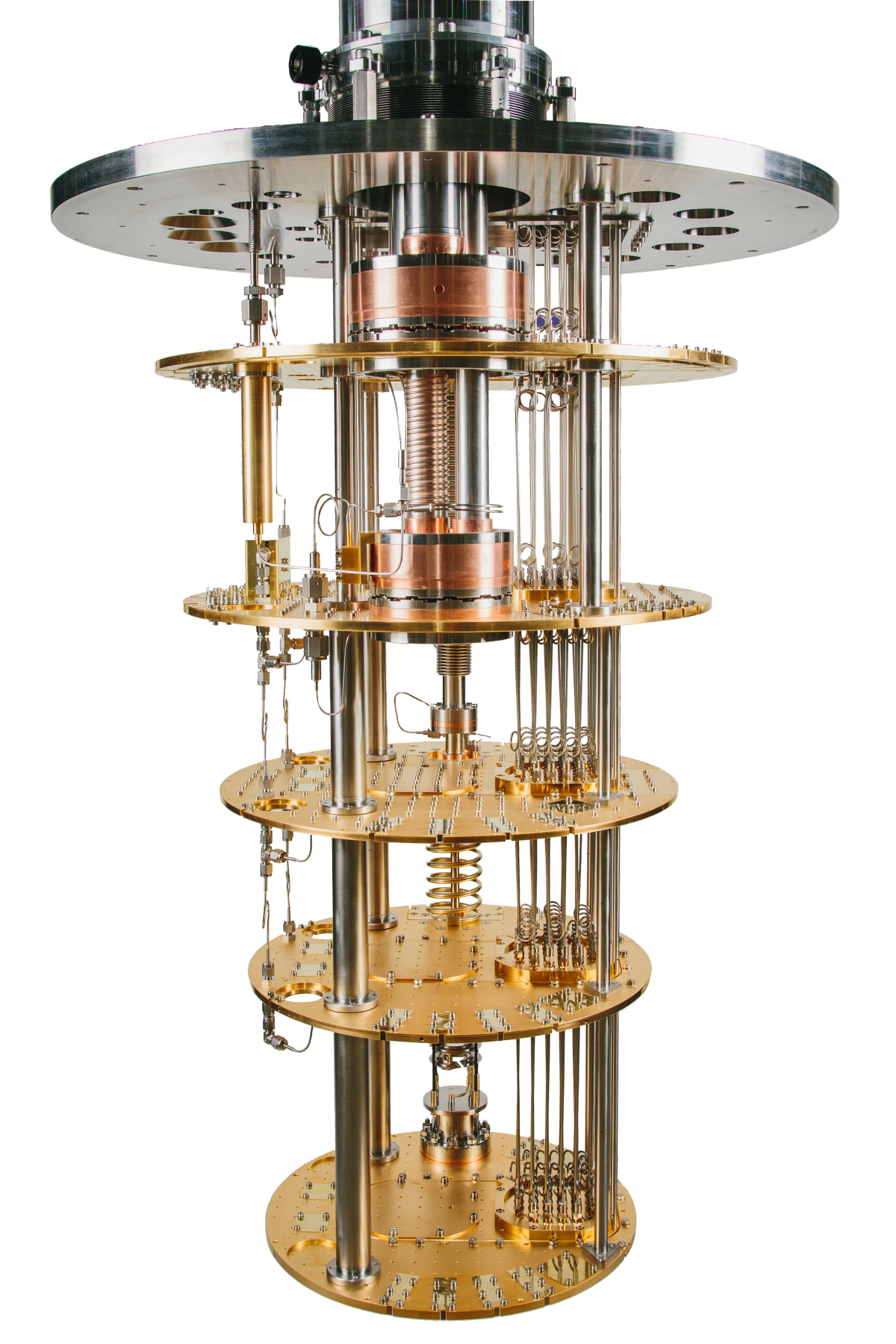
In practice, they operate at
Mechanical
Before we analyze the Hamiltonian and its eigenvalues, let's pause to compare our quantized LC circuit with the mechanical spring system introduced earlier in the lecture.
Drawing on this analogy helps build intuition for how the LC circuit oscillates.
| Quantity | Mechanical (spring) | Electrical (LC) |
|---|---|---|
| Coordinate | Position |
Flux |
| Conjugate Momentum | Charge |
|
| Mass | Capacitance |
|
| Restoring Force | Spring constant |
Inverse Inductance |
| Commutator |
Fock States of the Quantum Harmonic Oscillator (QHO)
Fock states are the energy eigenstates of the quantum harmonic oscillator (QHO) Hamiltonian and represent distinct, quantized energy levels.
The Hamiltonian can be written in terms of ladder operators as
When this Hamiltonian acts on a Fock state
Remember that
Even in the absence of excitations (
This relates to the two constants
Statistical Mean Values: Due to the symmetry of Fock states, both the mean flux (
Similarly, for charge, we have
Variance and Zero Point Fluctuations (ZPF): Although the mean values are zero, the fluctuations, measured by the variance, are nonzero and increase with the excitation number
For example, the variance of flux is given by
In the ground state (
Derive the expression
We have seen that the system's total energy is divided between the inductive and capacitive forms.
The inductive energy is given by
The capacitive energy is
The variance
As we've discussed, Fock states provide a quantized description of energy in the oscillator, with their wavefunctions displaying characteristic spreads in flux and charge due to zero-point fluctuations.
However, to visualize and compare how these quantum states occupy phase space relative to their classical analogs, it is helpful to introduce alternate representations.
Particularly, we'll use quasi-probability distributions like the Husimi Q-function.
In the following section, we will explore how both classical and quantum states are represented in phase space and better understand the transition from deterministic orbits to the inherently probabilistic nature of quantum mechanics.
Phase Space Representations: Classical vs. Quantum
In classical mechanics, the state of an oscillator with fixed energy traces a precise elliptical trajectory in the
As a result, a quantum state is described not as a point but as a "cloud" of probability.
The Husimi Q-function provides a valuable mathematical tool for visualizing this quasi-probability distribution. It is defined by the expression
and represents the expectation value of the density matrix projected onto a coherent state
For the ground state
Fock states
The Transmon Qubit
We begin this section by recalling some important dates of this field of research that started more than 40 years ago.
Indeed, the demonstration of the quantized energy levels of a Josephson junction was first achieved in 1985 4 by John Martinis, Michel Devoret, and John Clarke[4].
That same year marked the creation of the quantronics group at CEA Saclay by Michel Devoret, Daniel Esteve, and Cristian Urbina.
Significant progress continued with the development of the Cooper[5] Pair Box in 1999 5.
This evolution ultimately led to the invention of the Transmon qubit in 2007 6.
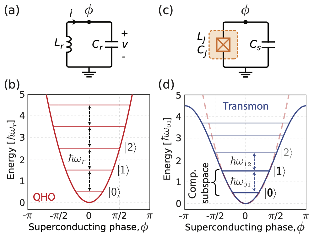
Why We Need Nonlinearity
A simple LC oscillator is not a qubit, a two-level system.
Its energy levels
If we try to drive a transition from
Imagine a ladder where every rung is spaced exactly 1 meter apart (harmonic oscillator). To climb it, you use a robot with fixed arms that can only reach exactly 1 meter.
If the robot tries to climb to the first rung, it succeeds perfectly. But because the next rung is also exactly 1 meter away, the robot will keep climbing to the second, third, or fourth rung when you only wanted it to stay on the first one.
To make a qubit, we need to "distort" the ladder. If we make the first rung 1 meter high, but the second rung only 0.9 meters away from the first, the robot can reach the first rung but will fail to reach the second. This unique spacing (anharmonicity) allows us to isolate just the bottom two levels (
To fix this, we need a non-linear circuit element that makes the energy spacing unequal (anharmonic).
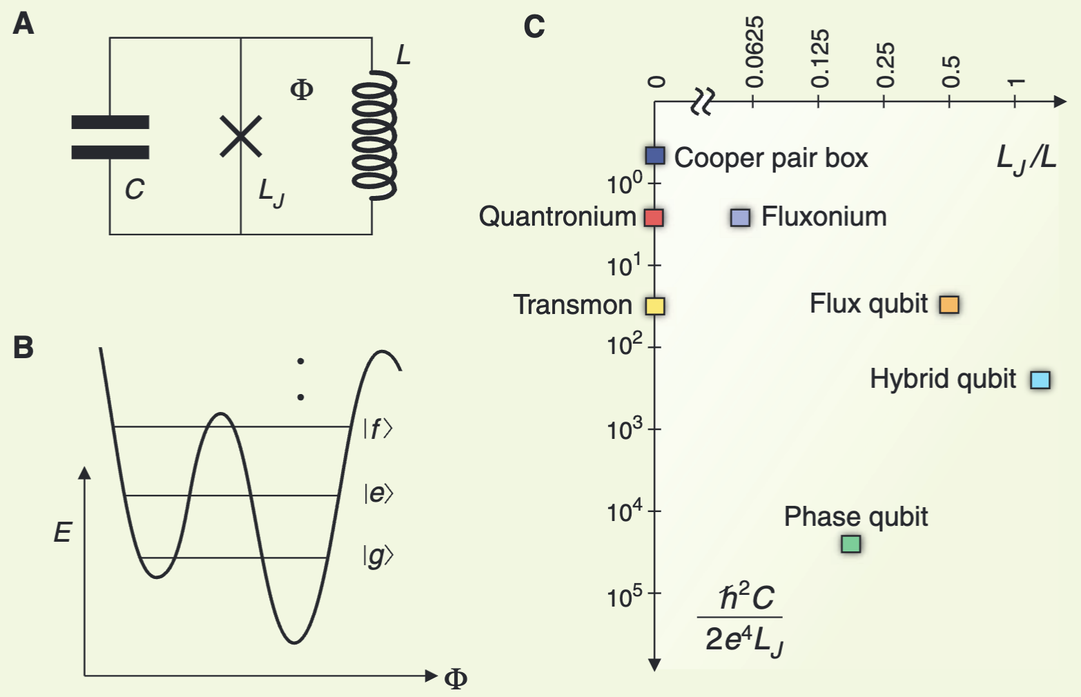
This element is the Josephson Junction, see Fig. extracted from 1.
Josephson Tunnel Junction
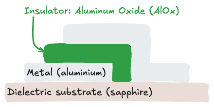
The Josephson Junction (JJ) acts as a non-linear inductor, see Fig..
The energy stored in the junction is given by
By Taylor expanding the cosine term, we can separate the energy into linear and non-linear components:
Expand
The linear term corresponds to a standard inductor, while the non-linear term provides the crucial anharmonicity necessary for qubit operation, to isolate the
Transmon Hamiltonian
A transmon consists of a Josephson Junction in parallel with a large shunting capacitor
The large capacitance reduces sensitivity to charge noise, making the qubit stable.
The full Hamiltonian is composed of two terms: the junction energy that we just saw (
The potential energy thus follows a cosine curve. For small oscillations near the bottom of the well, it behaves like a harmonic oscillator with energy
The key innovation of the Transmon is the large capacitor in parallel. In our mechanical analogy, this is like making the mass of the pendulum very heavy.
Why do this? A heavy mass is hard to disturb. In the quantum world, this makes the qubit much less sensitive to "charge noise", aka random fluctuations in the electric environment. This stability comes at a cost: the anharmonicity (the difference between energy levels) gets smaller, but it's a worthy trade-off for a qubit that lives much longer (
Let's get a semi-classical intuition from the Phase Space Picture.
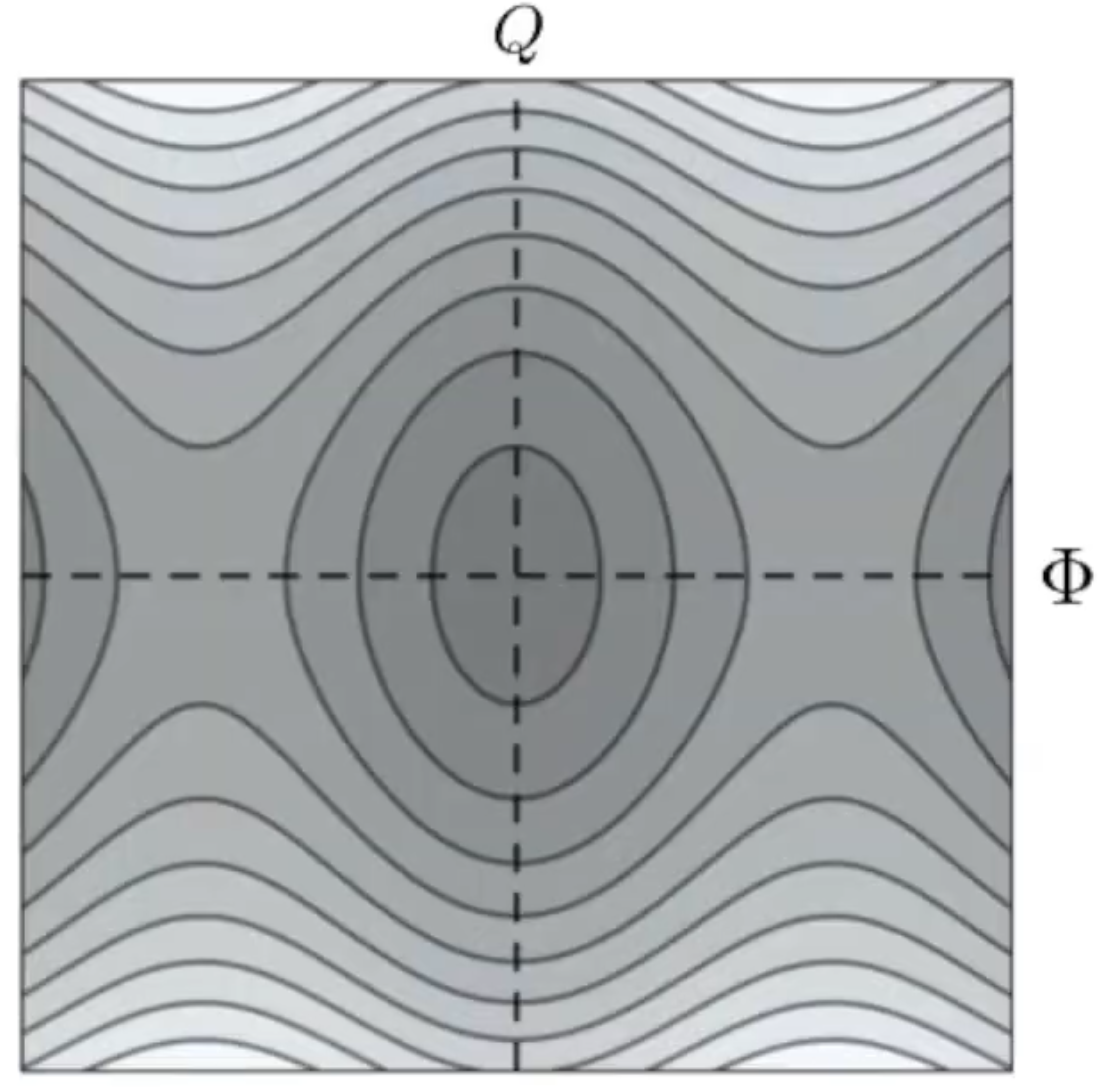
We can describe the system using the Hamiltonian
For a standard harmonic oscillator, the energy levels would be:
In phase space (
However, the cosine term in the Transmon Hamiltonian deforms these trajectories as the energy increases, leading to anharmonicity (uneven spacing between energy levels), see Fig..
Quantum Treatment of the Transmon
Having established the semiclassical and circuit-level understanding of the transmon, we now move to its full quantum description.
This section will show how to quantize the transmon Hamiltonian, treat the effects of its nonlinearity, and reveal how the anharmonicity arises, at the origin of the qubit behavior.
We start from the Taylor-expanded Hamiltonian:
that we rewrite using the creation and annihilation operators
with
Expanding the
Imagine pushing a child on a swing. You naturally push at the moment the swing is moving away from you. This effectively adds energy.
Now imagine you are jittering your hands back and forth really fast while pushing, adding some kind of vibration or shaking. These fast jitters don't really move the swing; they average out to zero over the course of a full swing. The RWA is the mathematical way of saying "ignore the fast jitters that don't match the swing's natural frequency." We keep only the terms that effectively transfer energy.
By expanding the terms, we find that
Expand
After grouping terms and accounting for the commutator
where:
is the Renormalization factor of the linear frequency due to Zero Point Fluctuations (ZPF). This is essentially a Lamb[6] shift due to ZPF. is the anharmonicity (also called Kerr nonlinearity), where (zero point fluctuation of the reduced magnetic flux).
We write the hamiltonian in its final form, called a Duffing Oscillator, using the number operator
Rearrange the expanded Hamiltonian to the form
Where
The energy levels in the system exhibit characteristic transitions.
The transition between the first excited state and the ground state is given by
The next transition, from the second excited state to the first, is
Typical parameter values for these transitions are
To first order perturbation theory, only the energy changes, not the wavefunctions (eigenvectors):
since
Let's take a numerical example:
For a standard transmon qubit setup, the following parameter values are used:
| Parameter | Symbol | Typical Value / Formula |
|---|---|---|
| Inductance | ||
| Capacitance | ||
| Bare Frequency | ||
| Josephson Energy | ||
| Charging Energy | ||
| Impedance | ||
| Anharmonicity | ||
| Qubit Frequency |
Calculate the anharmonicity
For the zero-point fluctuations, the ratio
For the flux quantum, we have
When the system is in the
Finally, in order to treat the system as a qubit, we restrict the Hilbert space and the operators to the subspace consisting of
The number operator can then be mapped from
Similarly, the lowering operator
Verify that the matrix representations of
We briefly mention that an entire zoo of superconducting qubits exist, depending on the ratio between the physical parameters, see Fig. taken from 7.
We can cite the Cooper pair box, flux qubit, phase qubit, quantronium, transmon, fluxonium, and hybrid qubit.
Qubit Control
We end this section by discussing three operations on the isolated transmon qubit: control via 1Q gates, measurement and 2Q gates.
In order to control the qubit, it is coupled to an input/output microwave drive line, typically a coaxial cable, using a capacitor that enables charge-to-charge coupling.
The drive Hamiltonian takes the form
The drive signal itself is expressed as
We say that the charge is coupled since we have
Show that
The drive signal and the qubit state can be expressed in the rotating frame to understand gate operations.
By writing
we can apply the Rotating Wave Approximation (RWA) to the drive (
Apply the unitary
In this interaction picture, the Hamiltonian reduces into two pieces: a first piece that depends on the detuning and sets the amplitude of the rotation at
This Hamiltonian allows for general rotations on the qubit by changing
An example is Rabi[7] Oscillations: a constant drive amplitude
Having only perfect control through coupling would be ideal.
However, control, noise, and dissipation are intrinsically linked.
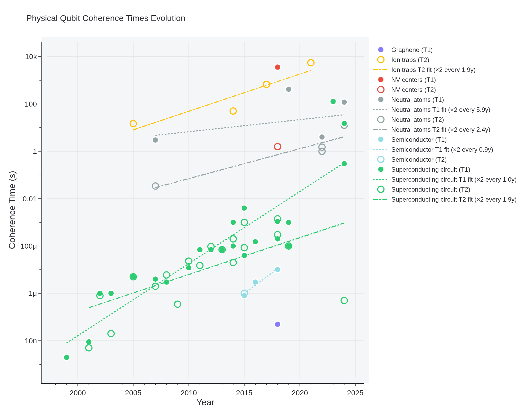
According to the Fluctuation-Dissipation Theorem, coupling to intrinsic I/O (input/output) channels leads to specific relaxation and decoherence times:
We saw progress in
Qubit Measurement Strategies
To measure the qubit, we could couple directly to an I/O transmission line.
This approach has the advantage of a simple setup.
However, it suffers from the "Purcell" effect (spontaneous emission), which limits
Instead, the qubit is coupled to a detuned microwave cavity (resonator) which is then coupled to the I/O line.
In the dispersive regime (where the qubit and resonator are detuned), the interaction Hamiltonian is:
This means the resonator's frequency shifts by
How do we measure the qubit without touching it? Imagine the qubit is a piece of glass inside the cavity. When the qubit is in state
This change shifts the resonant frequency of the cavity. By sending a tone into the cavity and seeing if it reflects or transmits, we can determine the "color" (frequency) of the cavity and thus deduce the state of the qubit. This is "dispersive" because it relies on the dispersion (frequency shift) rather than absorption of energy.
Using second-order perturbation theory on the Jaynes-Cummings Hamiltonian, derive the dispersive shift
This Quantum Non-Demolition (QND) setup inhibits spontaneous emission. The measurement mechanism relies on the fact that the reflection of the I/O line at the resonator depends on the qubit's state. Oscillators are used for both readout and facilitating 2-qubit (2Q) gates.
Two Coupled Transmon Qubits
We saw how to perform single qubit gates on the transmon and how to measure its state.
The last piece is how to generate entanglement between tramson qubits.
When two transmons (or a transmon and a resonator) are coupled via a capacitor, the system is described by individual Hamiltonians:
- Qubit 1:
- Qubit 2:
The total Hamiltonian can be separated into linear and non-linear parts (
The linear part corresponds to the Hamiltonian of the two QHO which is
The non-Linear Part is Derived from the Taylor expansion of the cosine potential for both transmons:
Because they are coupled, the physical fluxes
In their quantized form, we look for fluxes as:
Notice that we could apply this method in the case of readout, where one system is the cavity (resonator) and the other is the qubit.
We have the following linear terms:
The non-linear coupling is expressed as:
From which we derive the standard dispersive regime interaction Hamiltonian.
One crucial limitation is that this approach is inherently limited to nearest-neighbor coupling.
Indeed, the two qubits must be connected via a physical electrical circuit, a capacitor in our example.
This implies that multiple
Bosonic Encoding
Bosonic Modes and Open Systems
Why Bosonic Modes?
After discussing how a two-level transmon can be encoded in a QHO, we revisit the QHO and its "ladder" of energy states.
Previously, we chose to encode our two-level system using the lowest two energy levels, which necessitated introducing anharmonicity so that these states could be manipulated independently without inadvertently affecting higher levels.
However, encoding information in a QHO is not limited to just its ground and first excited states.
Instead, any two specific states among the infinite set of resonator states can be selected, including states constructed as clever superpositions.
We denote these specially chosen states as
For instance, we could have chosen specific Fock state combination like
This approach to encoding information in QHO or bosonic modes is known as a bosonic code.
Bosonic modes provide several significant advantages.
First, they offer hardware efficiency because information can be encoded in high-dimensional Hilbert spaces.
Second, high-Q resonators serving as bosonic modes can exhibit much longer coherence times than traditional qubits, resulting in longer lifetimes for the encoded information.
Third, established techniques for microwave state manipulation enable robust control of these bosonic modes.
Finally, the errors encountered in such systems are typically simpler, with photon loss being the predominant type of error.
Moving from the ideal QHO to open systems requires us to account for environmental interactions such as photon loss and dephasing.
Our first step is to write down the equation of motion that describes these open systems, introduce an nice visualization tool, and examine different examples of QHO behavior.
The Lindblad Master Equation
First, to describe the evolution of a state in a QHO, the "simple" Schrödinger[8] equation is not enough.
We have to include environmental interactions.
The evolution of the density matrix
Where the Lindbladian dissipator is given by
In this context,
The new operators
Verify that the Lindblad equation preserves the trace of the density matrix (
Coherent States
Before introducing the visualizing tool for quantum states of a QHO in phase space, it is essential to introduce the class of coherent states, which are the "most classical" states of the quantum harmonic oscillator.
A coherent state
where
Mathematically, in the Fock state basis, a coherent state is expressed as a superposition of number states weighted by Poissonian amplitudes:
The probability to find
Show that the probability distribution
Physically, a coherent state can be created by displacing the vacuum state
The displacement operator is defined as:
Thus,
A coherent state
In a coherent state, this fuzzy ball swings back and forth without spreading out or changing shape. It stays "coherent." The distance from the center tells you the number of photons (energy), while the angle tells you the phase of the oscillation.
Prove that applying the displacement operator
Hints:
- Consider the Baker-Campbell-Hausdorff (BCH) formula for operator exponentials.
- Write
and act with on this state. - Show explicitly that
.
One idea that will become crucial in the next section is to focus on the parity of such states.
Understanding the parity of coherent states gives us physical intuition for phase space representations like the Wigner function.
The parity operator is defined as
The average parity of a quantum state is the difference between the probability of having an even number of photons and an odd number of photons:
For the vacuum state
But what is the parity of a coherent state far from the vacuum state?
For a coherent state with large energy (large
Because this distribution is smooth and spreads across many integers, the probability of having
Therefore, the positive and negative terms in the parity sum cancel each other out:
Mathematically, the expectation value of parity for a coherent state is
This will explain why the Wigner function (understood as a parity expectation) of the vacuum state
The Wigner Function Definition and Intuition
In the previous sections, we referred to phase space several times to visualize the possible trajectories of the system.
Now, to fully characterize quantum states of a QHO in phase space, a nice tool is the Wigner[9] function, which serves as a powerful visualization tool for understanding state evolution.
The Wigner function
In the context of a Quantum Harmonic Oscillator (QHO), regions where the Wigner function takes on negative values directly indicate the presence of quantum behavior.
Think of the Wigner function as a topographic map of the quantum state in phase space.
- Hills (Positive): Where the particle is likely to be found (like a probability distribution).
- Valleys (Negative): This is where it gets weird. Negative probabilities don't exist in the classical world. A negative value in the Wigner function is a smoking gun for quantum interference effects. It's the signature that says "this is definitely not just a classical noisy system."
Mathematically, the Wigner function is defined as
Show that the integral of the Wigner function over all phase space is normalized to unity:
From this expression alone it can be hard to grasp the physics of it.
From an intuitive perspective, the value of the Wigner function at a given complex point
Here, the parity operator is given by
The displacement operator is
For instance, the operator transformation
Similarly, applying the displacement operator to the vacuum state as
We will use Wigner representations of states a lot in this last section, starting with some simple examples of dissipation.
The displacement operator
Examples of Dissipation
To illustrate Wigner representation from Lindblad master equations and to introduce the cat qubit as our first example of bosonic code, we first look at cavities with photon loss.
Simple Photon Loss
Photon loss or loss of excitation from the cavity to the environment is the predominant type of error in QHO.
When the dissipation operator is
As time progresses, the system settles into the vacuum state independently of the initial state, which means
In the phase space representation, such as a Wigner function, the state can be seen spiraling toward the origin.
Locality in Phase Space of the Damped Cavity
An important point that motivates the study of bosonic modes is the locality of errors in phase space, such as photon loss.
The Wigner representation indeed reveals that for QHO, errors occurring at high rates are usually the result of local processes within phase space.
Mathematically, this behavior is captured by the Fokker-Planck[10] Equation.
In the case of a damped cavity characterized by a loss rate
The diffusion term leads to a broadening of the distribution over time.
At the same time, global drift acts to pull the state back toward the vacuum state
Encoding information in the Hilbert space of the QHO is a form of non-local encoding well suited to fight local errors, just like quantum error correction, as we will see in the next lectures.
Driven Damped Cavity
Let's look at another example of QHO dynamics, this time a bit more complex.
When the system features both a drive Hamiltonian, given by
Here, the displacement
To see this, consider the outlined mathematical derivation.
First, we expand the driven master equation:
By carrying out algebraic manipulations, this master equation can be simplified and rewritten in terms of the dissipator for a displaced operator:
This driven-damped system stabilizes to a coherent state
Cat Code: Two-Photon Driven Damped QHO
Encoding information is not possible in a single photon driven damped oscillator, because the kernel of its effective dissipation consists of only a single state.
To enable information encoding, we require the kernel of the dissipative dynamics to have higher dimension.
We can achieve this by squaring the terms in the Lindblad master equation, which intuitively results in a two-dimensional kernel.
Such a configuration gives rise to the formation of Schrödinger Cat states.
The Hamiltonian for this system is given by
The dissipation operator takes the form
The equation of motion is expressed as
At steady state, the displacement is
In phase space, the system stabilizes into two distinct lobes in the
Physically, these systems are realized by coupling multiple resonators to induce nonlinear interactions through 4-wave mixing.
The experimental setup includes two coupled oscillators, denoted as modes
The drive Hamiltonian is
The effective Hamiltonian describing this interaction is
For simplicity, this can be modeled with the operators mentioned above:
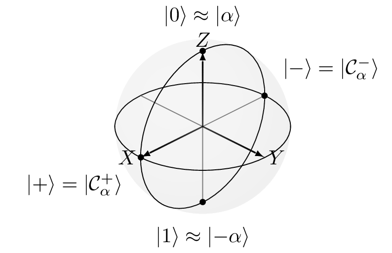
In this system, two coherent states,
Why "Cat"? In Schrödinger's thought experiment, the cat is in a superposition of "Dead" and "Alive." These are two macroscopic, distinguishable states.
Here, our "Dead" and "Alive" states are
The even cat state,
The odd cat state,
Show that
These logical states represent a qubit with its associated Bloch sphere illustrated in figure Fig..
| Logical State | Notation | Phase Space Representation |
|---|---|---|
| Zero |  |
|
| One |  |
|
| Plus | 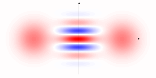 |
|
| Minus | 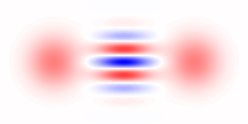 |
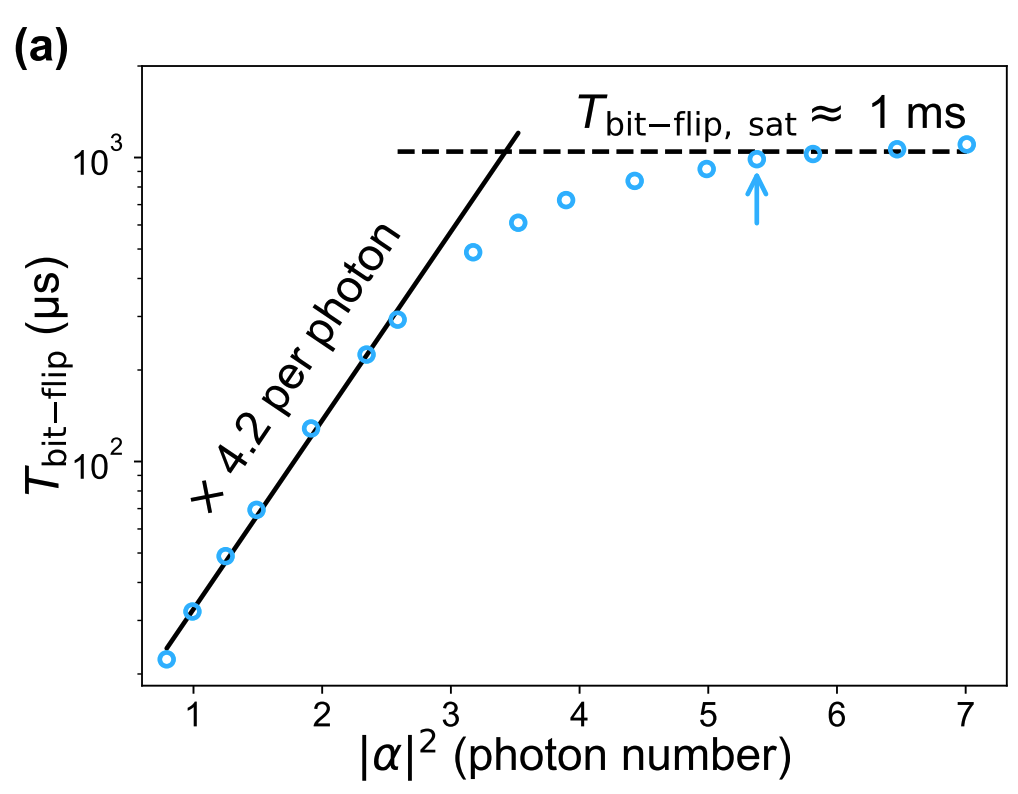
A key objective is to suppress bit-flip (
Using coherent states that are well separated in phase space causes their overlap, which produces errors, to become exponentially small. The overlap between two coherent states
As
Hence, the bit-flip time
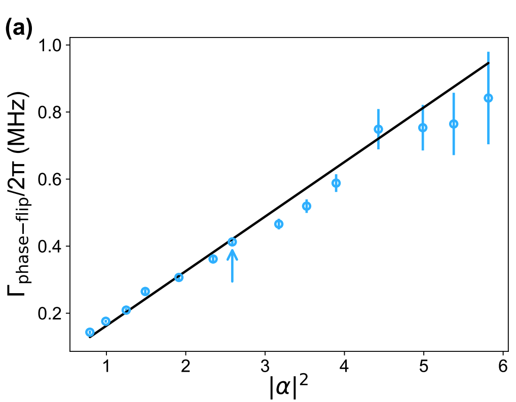
In contrast, the phase-flip rate
Indeed, increasing
The ratio between phase-flip and bit-flip error probabilities has reached values of up to
Calculate the overlap
One possible strategy for a Fully Protected Qubit involves considering simpler quantum error correction code, specifically 1D instead of 2D codes.
This topic will be discussed in detail in the QEC lecture.
Other bosonic qubits exist, but we are not going to discuss them in this lecture.
We only mention that Cat code belongs to a broader family of Rotationally Symmetric Codes (rotational symmetry referring to the Wigner representation).
This family includes the 4-Component Cat Code, where four coherent states are used to encode the logical information (
Another code robust against single photon loss is the much simpler Kitten code defined with
Finally, we have to mention a translationally symmetric code known as the GKP (from Gottesman, Kitaev and Preskill) code.
This code encodes a qubit in grid states of light and is robust against small displacements in phase space.
We end this section by focusing on operations that preserve the noise bias of cat qubits, called bias preserving operations.
Bias Preserving Operations
Having described how bosonic modes are encoded, we now discuss the process of performing operations on them, focusing in particular on the cat code.
When working with qubits that have biased noise, it is essential that operations do not convert the suppressed error type into a more dominant one.
A standard Hadamard gate is thus not suitable in this context because it swaps
Instead, only certain operations are permissible:
The parity state preparation
A
where
To effectively maintain protection of the code space, it is required that
To implement a logical
The evolution of the system during this operation follows the equation
in which
The mechanism relies on physically rotating the state in the complex plane over a period
During this rotation, strong dissipation as described by the
The CNOT gate is realized as a conditional operation that depends on the state of the control qubit, labeled as qubit 1.
In operator form, the CNOT can be expressed as
An equivalent projection representation is
This means that if the control qubit is in the
The evolution of the system during the CNOT gate is governed by the equation
where
Nobel prize in 1973 for his theoretical predictions of the properties of a supercurrent through a tunnel barrier ↩︎
Nobel prize in 1933 for the discovery of new productive forms of atomic theory ↩︎
Nobel prize in 1932 for the creation of quantum mechanics ↩︎
Clarke, Devoret and Martinis obtained Nobel prize in 2025 for experiments demonstrating macroscopic quantum mechanical tunnelling and energy quantisation in an electric circuit ↩︎
Nobel prize in 1972 for his jointly developed theory of superconductivity, usually called the BCS-theory ↩︎
Nobel prize in 1955 for his discoveries concerning the fine structure of the hydrogen spectrum ↩︎
Nobel prize in 1944 for his resonance method for recording the magnetic properties of atomic nuclei ↩︎
Nobel prize in 1933 for the discovery of new productive forms of atomic theory ↩︎
Nobel prize in 1963 for his contributions to the theory of the atomic nucleus and the elementary particles ↩︎
Max Planck received the Nobel prize in 1918 for the discovery of energy quanta ↩︎
References
- 1.
- Krantz, P; Kjaergaard, M; Yan, F; Orlando, T; Gustavsson, S; Oliver, W . A Quantum Engineer's Guide to Superconducting Qubits. Applied Physics Reviews 6 (2) , 021318 (2019) . doi:10.1063/1.5089550
- 2.
- Joshi, A; Noh, K; Gao, Y . Quantum information processing with bosonic qubits in circuit QED. Quantum Science and Technology 6 (3) , 033001 (2021) . doi:10.1088/2058-9565/abe989
- 3.
- Dirac, P; Dirac, P . The Principles of Quantum Mechanics. (1981) .
- 4.
- Martinis, J; Devoret, M; Clarke, J . Energy-Level Quantization in the Zero-Voltage State of a Current-Biased Josephson Junction. Physical Review Letters 55 (15) , 1543–1546 (1985) . doi:10.1103/PhysRevLett.55.1543
- 5.
- Nakamura, Y; Pashkin, Y; Tsai, J . Coherent control of macroscopic quantum states in a single-Cooper-pair box. Nature 398 (6730) , 786–788 (1999) . doi:10.1038/19718
- 6.
- Koch, J; Yu, T; Gambetta, J; Houck, A; Schuster, D; Majer, J; Blais, A; Devoret, M; Girvin, S; Schoelkopf, R . Charge-insensitive qubit design derived from the Cooper pair box. Physical Review A 76 (4) (2007) . doi:10.1103/physreva.76.042319
- 7.
- Devoret, M; Schoelkopf, R . Superconducting Circuits for Quantum Information: An Outlook. Science 339 (6124) , 1169–1174 (2013) . doi:10.1126/science.1231930
- 8.
- Le Régent, F . Awesome Quantum Computing Experiments: Benchmarking Experimental Progress Towards Fault-Tolerant Quantum Computation. (2025) . doi:10.48550/arXiv.2507.03678
- 9.
- Lescanne, R; Villiers, M; Peronnin, T; Sarlette, A; Delbecq, M; Huard, B; Kontos, T; Mirrahimi, M; Leghtas, Z . Exponential suppression of bit-flips in a qubit encoded in an oscillator. Nature Physics 16 (5) , 509–513 (2020) . doi:10.1038/s41567-020-0824-x